

Добавил:
Upload
Опубликованный материал нарушает ваши авторские права? Сообщите нам.
Вуз:
Предмет:
Файл:
Скачиваний:
67
Добавлен:
14.05.2015
Размер:
3.21 Mб
Скачать

Настройка приемника
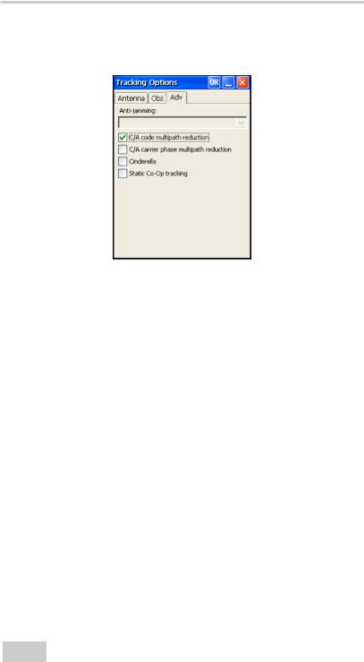
10.Выберите вкладку Advanced. Задайте следующие параметры и нажмите OK (Рис. 3-14 на стр. 3-15).
•Anti-jamming – при наличии в приемнике такой функции включается подавление помех в узком отрезке диапазона при приеме сигналов GPS, GLONASS, L1, L2. Отрезок диапазона, где присутствуют помехи, определяется автоматически или задается вручную.
•C/A code multipath reduction – когда отмечено это поле, то применяется специальная методика обработки сигнала, позволяющая подавить многолучевость в кодовых измерениях.
•C/A carrier phase multipath reduction – когда отмечено это поле, то применяется специальная методика обработки сигнала, позволяющая подавить многолучевость в фазовых измерениях.
•Cinderella – когда отмечено это поле, то включается опция Cinderella, которая на 24 часа открывает доступ ко всем возможным функциям приемника. Эта опция включается каждый второй вторник в полночь по времени GPS.
•Static Co-Op tracking – когда отмечено это поле, то приемник, работающий в режиме статики, принимает со спутников сигналы с низким уровнем “сигнал-шум”. Эту опцию следует использовать только в случаях, когда антенна приемника остается совершенно неподвижной на протяжении всей съемки. Любое
|
GRX2 — Руководство по эксплуатации |
3-57 |
Конфигурация GRX2
смещение может привести к тому, что связь со спутником будет потеряна.
Рис. 3-14. Настройка дополнительных параметров
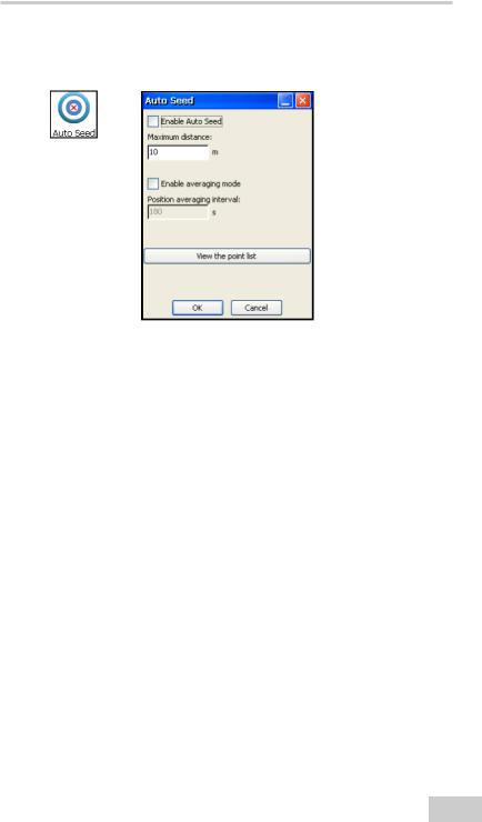
11.Для настройки базового приемника нажмите значок Auto Seed и задайте следующие параметры (Рис. 3-15 на стр. 3-16), после чего нажмите OK.
•Enable Auto Seed (не рекомендуется при проведении съемки): когда отмечено это поле, то включается функция авторежима для базовой станции, которая позволяет быстро установить приемник над точкой и начать RTK съемку без использования внешнего интерфейса и изменения настроек базового приемника. Последний автоматически выбирает новое местоположение по результатам осреднения координат, полученных в автономном режиме работы, и сохраняет их для последующих наблюдений.
•Maximum distance: если на точке ранее проводились измерения, и текущие координаты приемника находятся в пределах заданного диапазона, то приемник выбирает точку из координат, хранящихся в памяти прибора.
•Enable averaging mode: когда отмечено это поле, то включается осреднение координат, определяемых в автономном режиме
|
3-58 |
||
|
GRX2 — Руководство по эксплуатации |
Настройка приемника
работы на точке стояния с интервалом, значение которого в секундах задается в поле Position averaging interval.
Рис. 3-15. Настройка базового приемника
•Нажмите кнопку View the point list, чтобы открыть список сохраненных точек, в котором содержатся следующие данные: имена, дата и время, координаты фазового центра антенны, была ли точка определена в автономном режиме и защищена ли она от удаления. Более подробно об автономном режиме
см. Справочное руководство GRX Utility.
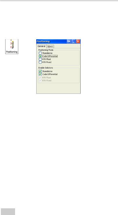
12.Для настройки ровера нажмите значок Positioning, задайте следующие параметры и нажмите OK (Рис. 3-16 на стр. 3-17).
•Positioning Mode – для съемок с постобработкой выберите параметр Standalone; для RTK съемок выберите параметр RTK float или RTK fixed.
•Enable Solutions – выберите тип решений, используемые при вычислении координат.
–Standalone – ровер вычисляет 3D координаты в автономном режиме без использования дифференциальных поправок.
–Code differential – вычисляются текущие координаты в дифференциальном режиме относительно базы с использованием только псевдодальностей.
–RTK float – вычисляются текущие координаты относительно базы с использованием как псевдодальностей, так фазовых
|
GRX2 — Руководство по эксплуатации |
3-59 |
Конфигурация GRX2
измерений; однако, поскольку при разрешении фазовой неоднозначности было получено не целое число, то такое решение называется “плавающим”.
–RTK fixed – вычисляются текущие координаты относительно базы в дифрежиме с разрешенной неоднозначностью.
Рис. 3-16. Настройка ровера
|
3-60 |
||
|
GRX2 — Руководство по эксплуатации |
Настройка приемника
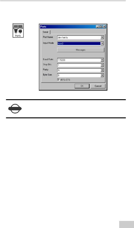
13.Для RTK съемки нажмите Ports, введите параметры СОМ порта, затем нажмите OK (Рис. 3-17 на стр. 3-18).
Рис. 3-17. Настройка портов
NOTICE
Для съемок с постобработкой используйте для этих параметров значения по умолчанию.
14.Чтобы сохранить настройки и закрыть окно, нажмите OK. Конфигурация приемника останется неизменной до тех пор, пока вы не измените ее с помощью программы GRX Utility или не очистите энергонезависимую память NVRAM. Более подробно о настройках приемника см. Справочное руководство GRX Utility.
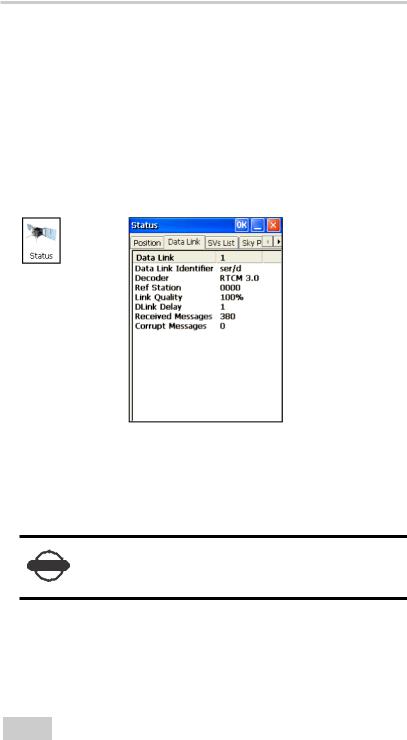
15.Для настройки RTK ровера нажмите Status (Рис. 3-18 на стр. 3-19), чтобы убедиться, что приемник принимает дифференциальные поправки. Как правило, приемник начинает выдавать координаты фазового центра антенны вместе с типом решения через 10-30 секунд. Однако, при использовании модемов Spread Spectrum и телефонов стандарта GSM на синхронизацию может уйти 60 секунд.
Во вкладке Data Link отражается статус полученных сообщений о дифференциальных поправках и содержится следующая информация:
•Качество связи в процентах (%);
|
GRX2 — Руководство по эксплуатации |
3-61 |
Конфигурация GRX2
•Время (в секундах) с момента приема последнего сообщения;
•Общее количество принятых нормальных сообщений (в зависимости от типа принятого сообщения)
•Общее количество принятых поврежденных сообщений (в зависимости от типа принятого сообщения)
Если приемник не получает (по какой-либо причине) дифференциальные поправки или ни один из портов не настроен на прием дифпоправок, поле Link Quality будет либо пустым, либо в нем будет стоять значение 100%.
Рис. 3-18. Окно Status — вкладка Data Link
16. Продолжите настройку других типов конфигураций или щелкните Device Disconnect, затем Device Exit, чтобы выйти из GRX Utility. Отключение приемника, перед тем как выйти из программы, обеспечивает корректную работу порта.
NOTICE
Прежде чем выйти из программы, отключите приемник, чтобы избежать возможных проблем
с работой СОМ порта.
Настройку приемников Sokkia можно также выполнять с помощью программы Spectrum Survey Field. См. Справочное
руководство Spectrum Survey Field или Руководство пользователя Spectrum Survey Field.
|
3-62 |
||
|
GRX2 — Руководство по эксплуатации |

Настройка приемника
|
3-20 |
GRX2 — Руководство по эксплуатации |

Глава 4
Работа с GRX2
После настройки конфигурации съемки установите каждый приемник, измерьте его высоту и приступайте к съемке. Индикаторная панель приемника позволяет легко контролировать запись данных измерений, изменять режимы работы приемника, просматривать по ходу съемки результаты измерений и данные спутников.
Установка приемника
Обычный комплект для GPS съемки состоит из базового приемника, который устанавливается над известной точкой, и ровера, который перемещается с точки на точку, выполняя измерения. После установки базы и ровера необходимо измерить высоту антенны.
Перед началом измерений проверьте, чтобы базовый приемник и ровер имели текущий альманах и последние эфемериды (см. “Получение альманахов и эфемерид” на стр. 2-14).
Шаг 1: Установка приемников
Первой устанавливается базовая станция, которая к моменту установки ровера, должна уже осуществлять измерения и передавать данные. Порядок установки базовой станции для съемки в RTK режиме и с постобработкой одинаков.
 Установка базовой станции и ее компонентов.
См. раздел “Для установки базовой станции” на стр. 4-1.  Установка ровера.
См. раздел “Для установки ровера” на стр. 4-3.
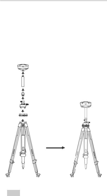
Для установки базовой станции (Рис. 4-1):
1. Установите штатив над точкой с известными координатами.
|
GRX2 — Руководство по эксплуатации |
4-1 |
Работа с GRX2
2.Закрепите на штативе стандартный трегер. Вставьте него адаптер трегера и затяните винты.
3.Вставьте в адаптер трегера адаптер призмы.
4.Прикрепите к адаптеру призмы переходник (10см).
5.Закрепите на переходнике (10см) приемник GRX2.
6.Вставьте в соответствующий разъем антенну.
7.Установите штатив так, чтобы его головка находилась в горизонтальной плоскости, и закрутите винты.
8.По мере необходимости установите другие принадлежности (например, внешний источник питания).
Приемник GRX 2
Переходник 10 см
Адаптер призмы Адаптер трегера
Стандартный трегер
Рис. 4-1. Установка штатива и приемника над точкой
|
4-2 |
GRX2 — Руководство по эксплуатации |
Соседние файлы в предмете [НЕСОРТИРОВАННОЕ]
- #
- #
- #
- #
- #
- #
- #
- #
- #
- #
- #

SokkiaSSF_um.book Page 1 Wednesday, August 12, 2009 10:34 AM

SokkiaSSF_um.book Page 2 Wednesday, August 12, 2009 10:34 AM

SokkiaSSF_um.book Page 1 Wednesday, August 12, 2009 10:34 AM
SokkiaSpectrum Survey Field
User’s Manual
Part Number 7010-0945
Rev A
©Copyright Topcon Positioning Systems, Inc.
August, 2009
All contents in this manual are copyrighted by Topcon Positioning Systems, Inc. All rights reserved. The information contained herein may not be used, accessed, copied, stored, displayed, sold, modified, published, or distributed, or otherwise reproduced without the expressed written consent from Topcon
Positioning Systems, Inc.

SokkiaSSF_um.book Page 2 Wednesday, August 12, 2009 10:34 AM
ECO#3642

TOC
SokkiaSSF_um.book Page i Wednesday, August 12, 2009 10:34 AM
Table of Contents
Chapter 1Introduction …………………………………………………. 1-1
Sokkia SSF on Controller ………………………………………… 1-2System Requirements ………………………………………… 1-2ActiveSync ………………………………………………………. 1-2Installing Sokkia SSF ………………………………………… 1-3Uninstalling Sokkia SSF ……………………………………. 1-7
Starting Sokkia SSF ………………………………………………… 1-7Demo Mode …………………………………………………………… 1-8
Chapter 2Getting Started …………………………………………….. 2-1
Opening Old Jobs …………………………………………………… 2-3Automatic Backup of Jobs ……………………………………….. 2-5Main Screen …………………………………………………………… 2-5
Title Bar ………………………………………………………….. 2-6Main Icons ……………………………………………………….. 2-7
Viewing Port Traffic ……………………………………………….. 2-8Accessing Help Files ………………………………………………. 2-11Before Surveying ……………………………………………………. 2-11
Chapter 3Preparation ………………………………………………….. 3-1
Global Navigation Satellite System (GPS+) Setup ……… 3-1Total Station (TS) Setup ………………………………………….. 3-2Level Setup ……………………………………………………………. 3-4
Chapter 4Creating a New Job ………………………………………. 4-1
Creating a GPS+ Configuration ………………………………… 4-3RTK Survey Configuration ………………………………… 4-6
NMEA Output Configuration ……………………….. 4-22
P/N 7010-0945 i

Table of Contents
SokkiaSSF_um.book Page ii Wednesday, August 12, 2009 10:34 AM
Laser Configuration …………………………………….. 4-23mmGPS+ Configuration ………………………………. 4-25PP Enabled RTK Survey Configuration …………. 4-26
Network RTK Survey Configuration ……………………. 4-28Survey Configuration for VRS and
FKP Methods ………………………………………….. 4-29NTRIP Internet Configuration ………………………. 4-30PP Enabled Network RTK Survey
Configuration …………………………………………… 4-38Network DGPS …………………………………………………. 4-39RT DGPS Survey Configuration …………………………. 4-39
PP Enabled RT DGPS Survey Configuration ….. 4-44PP Kinematic and PP DGPS Survey Configurations 4-45PP Static Survey Configuration …………………………… 4-49
Creating a Total Station Configuration ………………………. 4-52Creating TS Configuration in Contractor Mode …….. 4-61
Configuration Setup ………………………………………………… 4-63Coordinate System …………………………………………….. 4-63
Adding a Projection ……………………………………… 4-65Adding a Custom Datum ………………………………. 4-68Adding a Geoid File …………………………………….. 4-70Grid to/from Ground Transformation …………….. 4-72
Units ………………………………………………………………… 4-74Display …………………………………………………………….. 4-76Alarms ……………………………………………………………… 4-77
Global Settings ……………………………………………………….. 4-78Customizing Menus …………………………………………………. 4-79Setting Background Images ……………………………………… 4-80
Chapter 5Importing and Exporting Data ………………………. 5-1
Importing Data ……………………………………………………….. 5-1Import from Job ………………………………………………… 5-1Import from Device …………………………………………… 5-6Import from File ……………………………………………….. 5-7
Points from Text File Formats ………………………. 5-8Points from AutoCAD DXF and AutoCAD
Drawing Files ………………………………………….. 5-10
Sokkia Spectrum Survey Field User’s Manualii

Table of Contents
SokkiaSSF_um.book Page iii Wednesday, August 12, 2009 10:34 AM
Points from TDS Coordinates Format ……………. 5-11Importing Lines ………………………………………….. 5-11Importing Multiple Data Types …………………….. 5-12Importing Roads …………………………………………. 5-13
Exporting Data ……………………………………………………….. 5-13Export to Job ……………………………………………………. 5-14Export to Device ………………………………………………. 5-18Export to File ……………………………………………………. 5-19
Points to Text File Formats ………………………….. 5-20Exporting Points to an ESRI Shape Format ……. 5-24Points to TDS Coordinates …………………………… 5-25Exporting Raw Data ……………………………………. 5-25
Exporting GPS Sessions to the Receiver ……………… 5-26
Chapter 6Storing Data …………………………………………………. 6-1
Editing Points …………………………………………………………. 6-1Storing Points …………………………………………………………. 6-7
Stand-alone Points …………………………………………….. 6-7Linework …………………………………………………………. 6-8Linework Package …………………………………………….. 6-9Area ………………………………………………………………… 6-11
Editing Codes …………………………………………………………. 6-12Editing Point Lists ………………………………………………….. 6-14Editing Layers ………………………………………………………… 6-16Editing Linework ……………………………………………………. 6-19Editing Areas …………………………………………………………. 6-21Operating Raw Data ……………………………………………….. 6-23Editing GPS Sessions ……………………………………………… 6-25Editing Objects from the
Main Map …………………………………………………………… 6-27
Chapter 7Designing Roads ………………………………………….. 7-1
Editing Roads …………………………………………………………. 7-2Editing Horizontal Alignments …………………………………. 7-4
Adding a Line …………………………………………………… 7-7Adding a Curve ………………………………………………… 7-8
P/N 7010-0945 iii

Table of Contents
SokkiaSSF_um.book Page iv Wednesday, August 12, 2009 10:34 AM
Adding a Spiral …………………………………………………. 7-9Intersection Point ………………………………………………. 7-11
Editing Vertical Alignments ……………………………………… 7-12Adding Vertical Grade ……………………………………….. 7-17Adding a Curve …………………………………………………. 7-17Adding Long Sections ……………………………………….. 7-18
Editing X-Sect Templates ………………………………………… 7-20Editing Cross-Section Sets ……………………………………….. 7-22Editing Roads from the Main Map …………………………….. 7-24
Chapter 8Surveying with Sokkia SSF …………………………… 8-1
Performing GPS+ Surveys ……………………………………….. 8-1Localization ……………………………………………………… 8-2Starting the Base ……………………………………………….. 8-6
Starting Base with Autonomous Position ……….. 8-8Config Radio ………………………………………………. 8-8Configure RE-S1 Repeater ……………………………. 8-9Multi Base ………………………………………………….. 8-10mmGPS+ Options ……………………………………….. 8-12
Initializing mmGPS+ …………………………………………. 8-13Transmitter Calibration ………………………………… 8-13Sensor Initialization …………………………………….. 8-16
Performing a Topo Survey ………………………………….. 8-18OmniSTAR Status ……………………………………….. 8-21Beacon Status ……………………………………………… 8-22Config BR-1 ……………………………………………….. 8-23
Performing an Auto Topo Survey ………………………… 8-24Known Point Initialization ………………………………….. 8-26Cross-Section ……………………………………………………. 8-27Find Station/Chainage ……………………………………….. 8-28Tape Dimension ………………………………………………… 8-29Performing a Static Survey …………………………………. 8-31
Performing Total Station Surveys ……………………………… 8-32Backsight Setup ………………………………………………… 8-32Sideshot Setup ………………………………………………….. 8-34Measuring Sideshot Sets …………………………………….. 8-36Angle/Distance Sets …………………………………………… 8-37
Sokkia Spectrum Survey Field User’s Manualiv

Table of Contents
SokkiaSSF_um.book Page v Wednesday, August 12, 2009 10:34 AM
Resection …………………………………………………………. 8-38Remote Benchmarks …………………………………………. 8-40Remote Control ………………………………………………… 8-42Cross-Section …………………………………………………… 8-43Find Station ……………………………………………………… 8-45Tape Dimension ……………………………………………….. 8-46Missing Line …………………………………………………….. 8-47Auto Topo ……………………………………………………….. 8-48Scanning ………………………………………………………….. 8-50
Scanning with Images ………………………………….. 8-51Scanning Without Images …………………………….. 8-58
Monitor ……………………………………………………………. 8-60Performing Level Surveys ……………………………………….. 8-62
Two Peg Test ……………………………………………………. 8-62Level Run ………………………………………………………… 8-64
Chapter 9Staking Out ………………………………………………….. 9-1
Stakeout a Point ……………………………………………………… 9-2Stakeout a Point in Direction ……………………………………. 9-8Stakeout a Point List ……………………………………………….. 9-10Stakeout a Line ………………………………………………………. 9-11Stakeout a Curve …………………………………………………….. 9-13Stakeout Line & Offset ……………………………………………. 9-15Stakeout Three Point Curve & Offsets ………………………. 9-20Stakeout Intersection & Offsets ………………………………… 9-22Stakeout Curve & Offsets ………………………………………… 9-25Stakeout Spiral & Offsets ………………………………………… 9-26Stakeout Roads ………………………………………………………. 9-28Stakeout Slope ……………………………………………………….. 9-31Stakeout Real Time Road ………………………………………… 9-34Stakeout DTM ……………………………………………………….. 9-37Stakeout Linework ………………………………………………….. 9-39Level Stakeout ……………………………………………………….. 9-40
DL Staking a Point ……………………………………………. 9-40DL Staking Point List ………………………………………… 9-42DL Staking Elevation ………………………………………… 9-42
P/N 7010-0945 v

Table of Contents
SokkiaSSF_um.book Page vi Wednesday, August 12, 2009 10:34 AM
Chapter 10COGO ………………………………………………………….. 10-1
Inverse …………………………………………………………………… 10-1Two-Point Inverse …………………………………………….. 10-1Inverse Point to Points List …………………………………. 10-2Inverse Point to Line ………………………………………….. 10-3
Point in Direction ……………………………………………………. 10-4Intersection …………………………………………………………….. 10-5Calculator ………………………………………………………………. 10-6Curve Solutions ………………………………………………………. 10-7
Curve ……………………………………………………………….. 10-8PI & Tangents …………………………………………………… 10-8Three Pt Curve ………………………………………………….. 10-9Radius & Points ………………………………………………… 10-10
Area ………………………………………………………………………. 10-11By Points ………………………………………………………….. 10-11Hinge ……………………………………………………………….. 10-12Line …………………………………………………………………. 10-14
Corner Angle ………………………………………………………….. 10-15Line Offset ……………………………………………………………… 10-15Curve Offset …………………………………………………………… 10-17Road Offset ……………………………………………………………. 10-18Adjust Points ………………………………………………………….. 10-19
Rotate ………………………………………………………………. 10-19Translate ………………………………………………………….. 10-20Scale ………………………………………………………………… 10-212D Transform ……………………………………………………. 10-22Traverse Adjustment ………………………………………….. 10-24
Traverse …………………………………………………………………. 10-25
Appendix AmmGPS Operations ……………………………………… A-1
Resection ……………………………………………………………….. A-1Field Calibration ……………………………………………………… A-8mmGPS Options ……………………………………………………… A-14
Sokkia Spectrum Survey Field User’s Manualvi

Table of Contents
SokkiaSSF_um.book Page vii Wednesday, August 12, 2009 10:34 AM
Appendix BUsing Topcon Link with Sokkia SSF Job Files .. B-1
Importing Sokkia SSF Jobs ………………………………… B-2Opening, Viewing, and Editing Sokkia SSF GPS Files B-3
Editing Instrument Height on the Station ……….. B-5View Points Coordinates ……………………………… B-5Save the File ………………………………………………. B-8
Converting a Sokkia SSF File to an AutoCAD File Format B-9
P/N 7010-0945 vii

Table of Contents
SokkiaSSF_um.book Page viii Wednesday, August 12, 2009 10:34 AM
Notes:
Sokkia Spectrum Survey Field User’s Manualviii

Preface
SokkiaSSF_um.book Page vii Wednesday, August 12, 2009 10:34 AM
Preface
Thank you for purchasing your Topcon® receiver, Sokkia® survey product or accessory (the “Product”). The materials available in this manual (the “Manual”) have been prepared by Topcon Positioning Systems, Inc. (“TPS”) for owners of Topcon products. This Manual is designed to assist owners with the use of software (the “Software”) to be used with the Product and its use is subject to these terms and conditions (the “Terms and Conditions”).
Terms and ConditionsUSE This product is designed to be used by a professional. The user should have a good knowledge of the safe use of the product and implement the types of safety procedures recommended by the local government protection agency for both private use and commercial job sites.
COPYRIGHT All information contained in this Manual is the intellectual property of, and copyrighted material of TPS. All rights are reserved. You may not use, access, copy, store, display, create derivative works of, sell, modify, publish, distribute, or allow any third party access to, any graphics, content, information or data in this Manual without TPS’ express written consent and may only use such information for the care and operation of your receiver. The information and data in this Manual are a valuable asset of TPS and are developed by the expenditure of considerable work, time and money, and are the result of original selection, coordination and arrangement by TPS.
NOTICE Please read these Terms and Conditions carefully.
P/N 7010-0945 vii

Preface
SokkiaSSF_um.book Page viii Wednesday, August 12, 2009 10:34 AM
TRADEMARKS Topcon®, HiPer®, Sokkia Spectrum Survey Filed™, Topcon Link™, Topcon Tools™, and Topcon Positioning Systems™ are trademarks or registered trademarks of TPS. Windows® and ActiveSync® are registered trademarks of Microsoft Corporation. Bluetooth® is a registered trademark owned by Bluetooth SIG, Inc. and is used by Topcon Positioning Systems, Inc. under license. Sokkia Corporation and the names of Sokkia Corporation products referenced herein are either trademarks or registered trademarks of Sokkia Corporation. Satel is a trademark of Satel, Oy. Other product and company names mentioned herein may be trademarks of their respective owners.
DISCLAIMER OF WARRANTY EXCEPT FOR ANY WARRANTIES IN AN APPENDIX OR A WARRANTY CARD ACCOMPANYING THE PRODUCT, THIS MANUAL AND THE RECEIVER ARE PROVIDED “AS-IS.” THERE ARE NO OTHER WARRANTIES. TPS DISCLAIMS ANY IMPLIED WARRANTY OF MERCHANTABILITY OR FITNESS FOR ANY PARTICULAR USE OR PURPOSE. TPS AND ITS DISTRIBUTORS SHALL NOT BE LIABLE FOR TECHNICAL OR EDITORIAL ERRORS OR OMISSIONS CONTAINED HEREIN; NOR FOR INCIDENTAL OR CONSEQUENTIAL DAMAGES RESULTING FROM THE FURNISHING, PERFORMANCE OR USE OF THIS MATERIAL OR THE RECEIVER. SUCH DISCLAIMED DAMAGES INCLUDE BUT ARE NOT LIMITED TO LOSS OF TIME, LOSS OR DESTRUCTION OF DATA, LOSS OF PROFIT, SAVINGS OR REVENUE, OR LOSS OF THE PRODUCT’S USE. IN ADDITION TPS IS NOT RESPONSIBLE OR LIABLE FOR DAMAGES OR COSTS INCURRED IN CONNECTION WITH OBTAINING SUBSTITUTE PRODUCTS OR SOFTWARE, CLAIMS BY OTHERS, INCONVENIENCE, OR ANY OTHER COSTS. IN ANY EVENT, TPS SHALL HAVE NO LIABILITY FOR DAMAGES OR OTHERWISE TO YOU OR ANY OTHER PERSON OR ENTITY IN EXCESS OF THE PURCHASE PRICE FOR THE RECEIVER.
LICENSE AGREEMENT Use of any computer programs or software supplied by TPS or downloaded from a TPS website (the “Software”) in connection with the receiver constitutes acceptance of these Terms
Sokkia Spectrum Survey Field User’s Manualviii

Terms and Conditions
SokkiaSSF_um.book Page ix Wednesday, August 12, 2009 10:34 AM
and Conditions in this Manual and an agreement to abide by these Terms and Conditions. The user is granted a personal, non-exclusive, non-transferable license to use such Software under the terms stated herein and in any case only with a single receiver or single computer. You may not assign or transfer the Software or this license without the express written consent of TPS. This license is effective until terminated. You may terminate the license at any time by destroying the Software and Manual. TPS may terminate the license if you fail to comply with any of the Terms or Conditions. You agree to destroy the Software and manual upon termination of your use of the receiver. All ownership, copyright and other intellectual property rights in and to the Software belong to TPS. If these license terms are not acceptable, return any unused software and manual.
CONFIDENTIALITY This Manual, its contents and the Software (collectively, the “Confidential Information”) are the confidential and proprietary information of TPS. You agree to treat TPS’ Confidential Information with a degree of care no less stringent that the degree of care you would use in safeguarding your own most valuable trade secrets. Nothing in this paragraph shall restrict you from disclosing Confidential Information to your employees as may be necessary or appropriate to operate or care for the receiver. Such employees must also keep the Confidentiality Information confidential. In the event you become legally compelled to disclose any of the Confidential Information, you shall give TPS immediate notice so that it may seek a protective order or other appropriate remedy.
WEBSITE; OTHER STATEMENTS No statement contained at the TPS website (or any other website) or in any other advertisements or TPS literature or made by an employee or independent contractor of TPS modifies these Terms and Conditions (including the Software license, warranty and limitation of liability).
SAFETY Improper use of the receiver can lead to injury to persons or property and/or malfunction of the product. The receiver should only be repaired by authorized TPS warranty service centers. Users should review and heed the safety warnings in an Appendix.
MISCELLANEOUS The above Terms and Conditions may be amended, modified, superseded, or canceled, at any time by TPS. The
P/N 7010-0945 ix

Preface
SokkiaSSF_um.book Page x Wednesday, August 12, 2009 10:34 AM
above Terms and Conditions will be governed by, and construed in accordance with, the laws of the State of California, without reference to conflict of laws.
Manual ConventionsThis manual uses the following conventions:
Example Description
File Exit Tap the File menu and tap Exit.
Enter Indicates the button or key labeled Enter.
Topo Indicates the name of a dialog box or screen.
Notes Indicates a field on a dialog box or screen, or a tab within a dialog box or screen.
TIP
Supplementary information that can help you configure, maintain, or set up a system.
NOTICE
Supplementary information that can have an affect on system operation, system performance, measurements, personal safety.
Sokkia Spectrum Survey Field User’s Manualx

Chapter 1
SokkiaSSF_um.book Page 1 Wednesday, August 12, 2009 10:34 AM
Introduction
Sokkia Spectrum Survey Field is Topcon Sokkia’s survey software available for hand-held controllers. Sokkia SSF is used for surveying, common layout, and GIS purposes including:
• Field data collection with Topcon GPS receivers; Sokkia, Topcon, Nikon and Leica Total Stations; and Topcon Digital Levels
• Roads design to create cross section templates, horizontal, and vertical alignments
• Stakeout designed objects
• Data conversions to a variety of file formats
• COGO calculations
Sokkia SSF installs on hand-held controllers that run Windows® CE operating system, such as Sokkia’s SHC2500, Topcon’s FC-2000, FC-2200, FC-2,500, FC-200 (with Windows Mobile 5 as well) and the integrated controller of GMS-2 and GMS-2 Pro. Topcon Link PC software is included with Sokkia SSF providing data integration with your current office software.
Also, Sokkia SSF 7.3 for Windows PC is available from Topcon’s website (www.topconpositioning.com). It will operate in a “demonstration” mode, allowing 25 points to be added to a job. To fully activate, a separate license must be purchased.
P/N 7010-0945 1-1

Introduction
SokkiaSSF_um.book Page 2 Wednesday, August 12, 2009 10:34 AM
Sokkia SSF on ControllerThe Sokkia SSF setup file will first be loaded onto a computer. To install Sokkia SSF onto the controller, use ActiveSync and a connection between the computer and the controller receiving the software download.
System RequirementsMinimum system requirements includes display 240×320 or 320×240 pixels, 64 MB RAM and 50 MB flash disk space (internal), and Windows® CE version 4.0 or higher.
ActiveSyncUsing ActiveSync, the controller can exchange data to a computer via USB cable.
1. Install ActiveSync in the computer and turn on the controller.
2. Connect the controller to the computer with the USB cable.
3. The controller will give the prompt, Connecting to Host.
4. The computer will prompt to set up a partnership or set up as a guest. Select the desired type of connection.
5. Once a connection has been established, the ActiveSync window will display on the computer.
NOTICEMicrosoft® ActiveSync® must be installed on the computer before installing Sokkia SSF.
TIP T
ActiveSync is available for free from the Microsoft website. (For downloading, access the website http://www.microsoft.com/windowsmobile/).
Sokkia Spectrum Survey Field User’s Manual1-2

Sokkia SSF on Controller
SokkiaSSF_um.book Page 3 Wednesday, August 12, 2009 10:34 AM
Installing Sokkia SSFUse the steps below to install Sokkia SSF onto the computer and controller.
1. Run SokkiaSSFSetup.exe on your computer. The Welcome screen displays (Figure 1-1).
Figure 1-1. Welcome Screen
2. Review the License Agreement (Figure 1-2).
Figure 1-2. License Agreement
• To accept the terms and continue, click the “I accept…” radio button and click Next.
• To decline the terms and quit installing Sokkia SSF, click the “I do not accept…” radio button and click Next. The
P/N 7010-0945 1-3

Introduction
SokkiaSSF_um.book Page 4 Wednesday, August 12, 2009 10:34 AM
InstallShield Wizard will close and Sokkia SSF will not install onto the computer or controller.
3. Select the features to install (Figure 1-3) and click Next.
Figure 1-3. Select Features to Install
4. After detecting device information, the wizard will begin the installation process.
5. Click Install to begin (Figure 1-4 on page 1-4).
Figure 1-4. Select Device
During the setup process, installation files are copied to the appropriate directories in your computer for ActiveSync to access.
Sokkia Spectrum Survey Field User’s Manual1-4

Sokkia SSF on Controller
SokkiaSSF_um.book Page 5 Wednesday, August 12, 2009 10:34 AM
Once finished, Sokkia SSF installation accesses ActiveSync and launches Add/Remove Programs to install Sokkia SSF in the controller (Figure 1-5).
Figure 1-5. Setup Status
If the controller is disconnected from the computer, the following screen displays (Figure 1-6). After connecting the controller and computer, click Retry to continue.
Figure 1-6. Install Completion Pending Controller Connection
ActiveSync starts the Add/Remove Programs process, which automatically detects an available installation and attempts to install it on the controller (Figure 1-7).
Figure 1-7. Data Retrieved From Mobile Device
6. Click Yes at the Installing Applications screen (Figure 1-8) to install Sokkia SSF into the default directory in the controller.
Figure 1-8. Installing Sokkia SSF
P/N 7010-0945 1-5

Introduction
SokkiaSSF_um.book Page 6 Wednesday, August 12, 2009 10:34 AM
If the controller does not have space available (Figure 1-9), a prompt will display to delete some files or programs to make room for Sokkia SSF, or to select other destination media.
Figure 1-9. Delete Files to Provide Space or Select Destination Media
7. After clicking Yes, ActiveSync copies the installation file (CAB file) from the computer to the controller.
Figure 1-10. Installation Complete
8. Once the transfer completes, follow the steps indicated on the controller’s screen to complete the Sokkia SSF installation.
Then the Setup Status screen displays to configure software installation. When finished, the InstallSheild Wizard Complete screen displays.
9. Click Finish to exit the install program.
10. Once the installation completes, the Sokkia SSF icon will display on the controller screen to start Sokkia SSF.
Sokkia Spectrum Survey Field User’s Manual1-6

Starting Sokkia SSF
SokkiaSSF_um.book Page 7 Wednesday, August 12, 2009 10:34 AM
Uninstalling Sokkia SSFThe Remove Programs tool in Windows CE or through the Add/Remove Programs tool in ActiveSync both uninstall (remove) Sokkia SSF from the controller.
Starting Sokkia SSFTo start Sokkia SSF, tap the Sokkia SSF icon on the controller screen and then press the Enter button. Upon initial startup, Sokkia SSF requires an access code to run (Figure 1-11). Contact a Topcon representative to acquire the necessary codes.
• Key Value – the identification number of the device; record to give to a Topcon representative.
• Activation IDs – the fields in which to enter the security codes received from a Topcon representative to activate either one or more of the following purchased modes: TS, Contractor, Robotic, GPS+, GIS (RT DGPS and PP DGPS), Roads, and mmGPS.
Figure 1-11. Security
TIP T
Removing Sokkia SSF from the controller is recommended before installing a software upgrade. Be sure to save all necessary job files first.
P/N 7010-0945 1-7

Introduction
SokkiaSSF_um.book Page 8 Wednesday, August 12, 2009 10:34 AM
Once entered, the access codes are saved in the hidden tsv_setup file in the directory where Sokkia SSF is located. To view existing codes or add a new code, tap the Sokkia Logo Help
Icon in the top-left corner of the screen and select the Activate Modules option.
Demo ModeUpon initial startup, a Demo version of Sokkia SSF is accessible after tapping either OK or Cancel on the Security screen. To run the demo version, tap OK on the warning message that displays (Figure 1-12).
Figure 1-12. Access to Demo
A full-featured demo version of Sokkia SSF will be available with operational data limited. This demo version can store up to 25 surveyed points and roads of 100 meters in length.
NOTICE
If upgrading existing Sokkia SSF of previous version to Sokkia SSF 7.3, the updated security key is required to complete the installation of this upgrade. For help in acquiring this security key, contact [email protected].
Sokkia Spectrum Survey Field User’s Manual1-8

Chapter 2
SokkiaSSF_um.book Page 1 Wednesday, August 12, 2009 10:34 AM
Getting Started
Sokkia SSF initially creates a Default job upon program installation. By default, all jobs are stored in the Job folder of the Sokkia SSF directory (Figure 2-1).
Figure 2-1. Open Job
• Open – makes the Default job current and opens the main screen (see Figure 2-6 on page 2-5).
• New – press to create a new job.
• Exit – quits the program.
• Browse – press to display browse directories to navigate to a desired job. Highlight the file and press OK to open the job from a remote directory (Figure 2-2 on page 2-2).
P/N 7010-0945 2-1

Getting Started
SokkiaSSF_um.book Page 2 Wednesday, August 12, 2009 10:34 AM
Figure 2-2. Open Existing Job
Sokkia SSF job’s files are made universal for using on controllers and personal computers. They have the tsj extension and need no conversion. You can transfer the *.tsj files between Windows CE and Windows PC databases directly using:
• A flash memory card and the PC card reader.
• Copy/paste procedure and ActiveSync connection.
• Topcon Link conversion utility installed on the PC (For detail see “Using Topcon Link with Sokkia SSF Job Files” on page B-1) and ActiveSync connection.
• Topcon Tools data processing software installed on the PC and ActiveSync connection.
• Sokkia SSF PC installed on the PC through import/export procedure from/to the Device and ActiveSync connection.
NOTICE
If the job has photo notes and the job history, be sure to copy these folders from the directory where the job resides. The copied job will work correctly but the previous job history will be lost.
Sokkia Spectrum Survey Field User’s Manual2-2

Opening Old Jobs
SokkiaSSF_um.book Page 3 Wednesday, August 12, 2009 10:34 AM
Opening Old JobsTo open a job created in a previous version of Sokkia SSF, click Job Open Job and tap the Browse button in the Open Job screen (Figure 2-2 on page 2-2). Then select the Ts6 Job Files (*.tsv) type, navigate to the desired tsv job, highlight it, and press OK (Figure 2-3).
Figure 2-3. Open Old Job
Tapping OK starts upgrading the job. Tap the Cancel button to abort upgrading. When the process is complete, the Cancel button turns into the Done button (Figure 2-4 on page 2-4), which opens the main screen for the upgraded job.
P/N 7010-0945 2-3

Getting Started
SokkiaSSF_um.book Page 4 Wednesday, August 12, 2009 10:34 AM
Figure 2-4. Job Upgrade Progress
After pressing the Done button, the *.tsv file turns into the *.tsj file and the Archive folder is created in the directory where the *.tsv file was located. This folder stores the .tsv jobs. If the job had a job history, a directory using the same name as the job, is also created to store the *.xml file with the job history (Figure 2-5).
Figure 2-5. Upgraded Jobs
Sokkia Spectrum Survey Field User’s Manual2-4

Automatic Backup of Jobs
SokkiaSSF_um.book Page 5 Wednesday, August 12, 2009 10:34 AM
Automatic Backup of JobsTo increase the reliability of work with jobs in Sokkia SSF, a backup copy is automatically created of the current job. This automatic renewal occurs about every ten minutes and is safely stored with a new name, i.e., file_name!YYY-MM-DD!.tsj.bak in a folder where the original *.tsj file is located.
Sokkia SSF will create a separate *.bak file for the current job every time the user opens the *.tsj file during the day with another date, but there cannot be more than three such files. If the *.tsj file is opened in subsequent days, the *.bak files previously formed will be overwritten to the ones with the newer dates.
If, for any reason, there is a problem opening the original *.ts file in Sokkia SSF, Topcon Tools, or Topcon Link, you can rename the latest *.bak file to the *.tsj file and try to open the renamed file.
Main ScreenThe Sokkia SSF main screen opens to work in the current job (Figure 2-6).
Figure 2-6. Sokkia SSF Main Screen
P/N 7010-0945 2-5

Getting Started
SokkiaSSF_um.book Page 6 Wednesday, August 12, 2009 10:34 AM
Title BarThe title bar of the main menu screen shows the name of the job that is open and the following icons (Table 2-1).
NOTICE
Sokkia SSF has two implementations of graphical user interface: Icon-based and List-based. By default, Sokkia SSF uses the Icon-based interface for fast and easy program operation. To toggle between the Icon and List Menus
(Figure 2-7), tap the Topcon Logo Help Icon in the top-left corner of the screen and select the Switch Menus option.
Figure 2-7. List Menu
Table 2-1. Title Bar Icons
Icon Description
Topcon Logo Help Icon – opens a pop-up menu giving access to the help files and some options specific to the current open screen
Controller Power Status Icon – shows power status
Reconnect Icon – reconnects other Bluetooth enabled devices to the controller
Connection Status Icon – shows connection status
Sokkia Spectrum Survey Field User’s Manual2-6

Main Screen
SokkiaSSF_um.book Page 7 Wednesday, August 12, 2009 10:34 AM
When within a menu option, the title bar displays the Topcon Logo Help Icon, the name of the open screen, and any system buttons (e.g., OK, Cancel, Finish) required for various operations (Figure 2-2 on page 2-2).
Main IconsThe Sokkia SSF Icon Menu on the main screen contains the following icons to provide access to job configuration, setup, display, and other jobsite functions, and to control data (Table 2-2):
Exit Icon – closes Sokkia SSF.
Return Icon – returns to the previous menu. When in a submenu, the Exit Icon turns into the this button.
Table 2-2. Main Menu Icons
Icon Description
Job – opens a submenu to create, open, delete a job or get information about an active job.
Configure – opens a submenu to create or change a configuration for a job. The icon changes its appearance and reflects the instrument set for use in the current job.
Export – opens a submenu to export job data to a new job, controller or a file.
Import – opens a submenu to import data from a job, controller or a file.
Edit Job – opens a submenu to edit the job data.
Edit Roads – opens a submenu to edit roads.
Table 2-1. Title Bar Icons (Continued)
Icon Description
P/N 7010-0945 2-7

Getting Started
SokkiaSSF_um.book Page 8 Wednesday, August 12, 2009 10:34 AM
Viewing Port TrafficTo view or save to a file incoming and outgoing traffic information of a controller port connected with Sokkia SSF, tap the Topcon Logo
Help Icon in the top-left corner of the Icon Menu screen and select the Port Data Logging option.
1. The Port Logging screen (Figure 2-8 on page 2-9) initially shows no data. Tap the Help Icon in the upper-left corner of the screen to open a pop-up menu and select one of the following options:
Setup Base – sets up GPS surveying.
Setup – sets up backsight and occupation points to start a Total Station survey.
Survey – opens a submenu to conduct a survey.
Stake – opens a submenu to stake out objects.
COGO – opens a submenu to calculate cogo tasks.
Map – opens the map for the current job.
Mode – switches between GPS and Total Station instruments for a survey.
Table 2-2. Main Menu Icons (Continued)
Icon Description
Sokkia Spectrum Survey Field User’s Manual2-8

Viewing Port Traffic
SokkiaSSF_um.book Page 9 Wednesday, August 12, 2009 10:34 AM
• Show incoming port data – check mark to view incoming data.
• Show outgoing port data – check mark to view outgoing data.
• Pause logging to screen – check mark to freeze the show of port traffic.
Figure 2-8. Port Logging
2. Check mark the Log to file box to save the data to a file. When the Save File screen (Figure 2-9) displays, assign a name and select a desired directory in the controller to save the file.
Figure 2-9. Save File
P/N 7010-0945 2-9

Getting Started
SokkiaSSF_um.book Page 10 Wednesday, August 12, 2009 10:34 AM
3. Tap OK to return to the Port Logging screen to view the data being saved to the file. The file name is also shown on the screen (Figure 2-10).
Figure 2-10. Logging to File
4. Check mark the Append box to add new data to the existing file on every start of Sokkia SSF. Press the OK button to confirm the operation.
Sokkia Spectrum Survey Field User’s Manual2-10

Accessing Help Files
SokkiaSSF_um.book Page 11 Wednesday, August 12, 2009 10:34 AM
Accessing Help FilesTap the Topcon Logo Help Icon in the top-left corner of any screen and select the Help option to open the general Sokkia SSF Help topics or a specific option for the current screen (Figure 2-11).
Figure 2-11. Sokkia SSF General Help Topics
Before SurveyingTo start surveying with Sokkia SSF, make several preparations of the available equipment (see “Preparation” on page 3-1), and create a job to perform specific tasks on the jobsite (see “Creating a New Job” on page 4-1).
The following sections describe the various Sokkia SSF functions to assist in getting started with the software.
NOTICE
Data corruption can occur during data collection if the controller is low on power. If a warning about low power level displays, save and close the current job.
P/N 7010-0945 2-11

Getting Started
SokkiaSSF_um.book Page 12 Wednesday, August 12, 2009 10:34 AM
Notes:
Sokkia Spectrum Survey Field User’s Manual2-12

Chapter 3
SokkiaSSF_um.book Page 1 Wednesday, August 12, 2009 10:34 AM
Preparation
Global Navigation Satellite System (GPS+) Setup
1. Plumb the survey antenna over the mark and switch on the receiver and the controller.
2. If the receiver and the controller are Bluetooth® enabled, set the Instrument type to GPS+ and check the Bluetooth option in Sokkia SSF (change this setting later in the Observation Mode screen).
To change the Bluetooth device that the controller is connected to, click the Reconnect icon in the upper right corner of the main screen.
3. If the receiver or the controller are not Bluetooth enabled, or the Bluetooth option is unchecked, connect the receiver to the controller with the cable and set the Instrument type to GPS+ in Sokkia SSF (change this setting later in the Observation Mode screen) (Figure 3-1 on page 3-2).
P/N 7010-0945 3-1

Preparation
SokkiaSSF_um.book Page 2 Wednesday, August 12, 2009 10:34 AM
Figure 3-1. Observation Mode – GPS
Total Station (TS) Setup1. Set up a tripod and then center the instrument over the mark.
2. By adjusting the tripod legs, center the cross hairs on the ground mark. Complete the process by using the leveling screws of the instrument so that the bubble indicates a level position. Switch on the total station and the controller.
3. If the total station and the controller are Bluetooth enabled, perform the following operations:
• In the total station – select Bluetooth option and set PIN code.
• In Sokkia SSF – set the Instrument type to Total Station in the Observation Mode screen; select the TS model and set the Connection mode to Bluetooth TS; enable the Bluetooth option in the Observation Mode screen.
Sokkia Spectrum Survey Field User’s Manual3-2

Total Station (TS) Setup
SokkiaSSF_um.book Page 3 Wednesday, August 12, 2009 10:34 AM
Figure 3-2. Observation Mode – Total Station
• Select the TS from the list of devices and set the Passkey value to PIN code (use the same code used in the total station).
To change the Bluetooth device that the controller is
connected to, click the Reconnect icon in the upper right corner of the main screen.
4. If the total station or the controller are not Bluetooth enabled, or the Bluetooth option is no check marked, connect the controller to the total station with the cable and set the Instrument type to Total Station in Sokkia SSF. Make sure the data transfer parameters in the total station correspond to those in the controller.
P/N 7010-0945 3-3

SokkiaSSF_um.book Page 4 Wednesday, August 12, 2009 10:34 AM
Level Setup1. Set up the instrument in a desired location, with the tripod legs
well spread and tapped into the ground.
2. By adjusting the tripod legs, roughly level the instrument. Complete the process by turning the level screws of the instrument to center the bubble within the circle. Switch on the instrument and the controller. Make sure that in the level the Out Module is set to RS-232C and the Measure option is selected from the Menu.
3. Connect the controller to the instrument with the cable and set the Instrument type to Total Station in Sokkia SSF.
Figure 3-3. Observation Mode – Level

Chapter 4
SokkiaSSF_um.book Page 1 Wednesday, August 12, 2009 10:34 AM
Creating a New Job
Follow the procedure below to begin working with Sokkia SSF and to create a New Job file.
1. Tap the Mode icon on the main screen and select the survey mode, GPS+ or Total Station, then tap OK (Figure 4-1). Choose Contractor Mode in Total Station survey mode for use by non-surveyors for Topo and Stakeout with total stations. Choose Total Station survey mode to configure a Level survey.
Figure 4-1. Observation Mode
2. To create a new job, tap Job New Job or tap the New button on the Open Job screen during initial startup (see Figure 2-1 on page 2-1). The New Job screen displays (see Figure 4-2 on page 4-2). Enter the Name of the job and corresponding information (that is, the name of the surveyor and any necessary comments). The date is stored automatically. Tap Next to move to the next screen. At any stage, select the Finish button to create a new job. See the following sections to create a new job for your mode of survey.
P/N 7010-0945 4-1

Creating a New Job
SokkiaSSF_um.book Page 2 Wednesday, August 12, 2009 10:34 AM
Figure 4-2. New Job
A Job file contains all the pertinent data for the work being done: settings of the performed work and information on the Survey Configuration.
A Survey Configuration is a set of settings, such as instrument parameters or radio settings, which are independent of the job (one configuration can be used on several jobs).
Survey configurations are stored in the Styles.tsstyles file in the Sokkia SSF directory.
3. By default all job files are stored in the Job folder of the Sokkia SSF directory. To change the location of the job being created, tap Browse on the New Job screen.
4. On the Survey Style screen (Figure 4-3 on page 4-3), select the Survey Configuration, for both the GPS+ and TS and tap Next. A Survey Configuration is a set of parameters that describe
NOTICE
Configuration settings are applied to the equipment only after opening a screen that measures and stores data in the job file.
NOTICETap Finish to make the new job current and use the settings from the previously open job.
Sokkia Spectrum Survey Field User’s Manual4-2

Creating a GPS+ Configuration
SokkiaSSF_um.book Page 3 Wednesday, August 12, 2009 10:34 AM
work conditions and depend upon the instrument used for the survey. The last open configuration will initially display.
Figure 4-3. Select Survey Configuration
See the following sections for procedures to create and edit survey configurations.
• “Creating a GPS+ Configuration” on page 4-3
• “Creating a Total Station Configuration” on page 4-52
Creating a GPS+ ConfigurationA new configuration is performed with the help of a Wizard.
When creating a GPS+ configuration, use pre-defined configurations or create new ones. The pre-defined configurations are listed in drop-down menus in the corresponding fields. In the GPS+ Configuration field, choose one of the pre-defined configurations or tap the List
button to create a new one or edit the parameters of an existing configuration. The Configurations screen displays.
NOTICEA user-friendly Wizard interface guides you through the steps to create a job configuration.
P/N 7010-0945 4-3

Creating a New Job
SokkiaSSF_um.book Page 4 Wednesday, August 12, 2009 10:34 AM
The Configurations screen contains a list of available GPS+ configurations (Figure 4-4). Either edit an existing configuration or create a new configuration.
Figure 4-4. Create/Edit a Configuration
1. To create a new configuration, tap the Add button (Figure 4-4).
2. On the Srv (survey) screen, choose the configuration type (either RTK, Network RTK, Real Time DGPS, Network DGPS, PP Static, PP Kinematic, or PP DGPS) and enter the name of the configuration (Figure 4-5).
Figure 4-5. Configure an RTK Survey
Sokkia Spectrum Survey Field User’s Manual4-4

Creating a GPS+ Configuration
SokkiaSSF_um.book Page 5 Wednesday, August 12, 2009 10:34 AM
For Network RTK, Network DGPS and RT DGPS survey modes, select the corrections type (Figure 4-6):
• VRS, FKP, Single Base or External Config for Network RTK and Network DGPS surveys.
• User Base, Beacon, SBAS, CDGPS, OmniSTAR-VBS or OmniSTAR-HP for RT and Network DGPS surveys.
Figure 4-6. Configure a Network RTK, Network DGPS, and RT DGPS
3. Post Processing – check mark and enable to configure a post processing survey type in either RTK, Network RTK, Network DGPS, RT DGPS mode.
4. mmGPS+ – check mark and enable to configure a mmGPS+ aided survey type in RTK and Network RTK mode.
5. Simulation Mode – check mark and enable to run Sokkia SSF GPS mode in a GPS simulation mode.
If Simulation Mode is selected, the Set Simulator icon becomes available in the Edit Job menu.
6. Depending on the mode, continue creating the configuration:
• For RTK see page 4-6.
• For Network RTK and Network DGPS see page 4-28.
• For RT DGPS see page 4-39.
• For PP Static survey mode see page 4-49.
P/N 7010-0945 4-5

Creating a New Job
SokkiaSSF_um.book Page 6 Wednesday, August 12, 2009 10:34 AM
• For PP Kinematic and PP DGPS see page 4-45.
RTK Survey ConfigurationReal time kinematic (RTK) surveying is used for topographic survey and stakeout, and is the most precise method of real-time surveying.
RTK requires at least two receivers (Base and Rover) collecting navigation data simultaneously and being linked via a communication system. The Base receiver is usually at a known location and serves as a reference station. The Base receiver collects carrier phase measurements, generates RTK corrections, and transmits this data to the Rover. The Rover receiver processes its carrier phase observations with the received corrections, computing its relative position. The closer the Rover is to the Base, the higher the probability of determining the integer values of ambiguities. Typically, the distance between the Base and Rover should not be more than 10-15 km.
To enable logging Base and Rover data for post processing in RTK survey, check and enable the Post Processing box in the Survey screen.
To configure a mmGPS+ aided RTK survey, check and enable the mmGPS+ box on the Survey screen.
After naming the configuration and selecting its type, tap Next on the Survey screen (Figure 4-5 on page 4-4) and continue below to finish the configuration for an RTK survey.
1. Set the parameters for the Base Receiver (Figure 4-7), and tap Next:
• Select Receiver Model of the Topcon receiver being used for survey. Select either GR-3, GMS-2/GMS-2 Pro, GMS X, NET G3, or Topcon Generic for any other Topcon receiver.
• Set Elevation Mask not to use data from satellites below this elevation.
• Select RTK Format of the Base receiver corrections transmitted to the Rover.
Sokkia Spectrum Survey Field User’s Manual4-6

Creating a GPS+ Configuration
SokkiaSSF_um.book Page 7 Wednesday, August 12, 2009 10:34 AM
• Select the TPS Antenna type from the list and set the height and its type (either Vertical measured to the antenna reference point or Slant measured to the antenna edge).
Figure 4-7. Configure Base Receiver
• Press the Peripherals button to enable the Multiple Ports option if needed to transmit data from different ports of the base receiver to use for peripherals (see Figure 4-8 on page 4-8).
• Select the Receiver Settings option from the Help Icon menu in the upper left corner of the Base Receiver screen to turn charging mode of the receiver battery off as needed.
• If it is necessary to use relative parameters at the base with CMR+ data transmission, select the Use Relative Calibrations option from the Help Icon menu.
Note: You can select this option when editing the base.
By default, Sokkia SSF uses Absolute calibration offsets for antennas.
P/N 7010-0945 4-7

Creating a New Job
SokkiaSSF_um.book Page 8 Wednesday, August 12, 2009 10:34 AM
Figure 4-8. Peripherals
2. Set the Base Radio – choose the modem to be used and its parameters, and tap Next (Figure 4-9).
Figure 4-9. Configure Base Radio
If Multiple Ports are set for peripherals (see Figure 4-8), depending on the number of ports selected, there can be several radios for correction data output.
3. Custom modems use a standard set of parameters: port, parity, the number of data bits, the baud rate and the number of stop bits. Tap the Default button to set default settings for the port.
AirLink GPRS, CDMA, CDPD1, CDMA2000, Generic, Sierra
Sokkia Spectrum Survey Field User’s Manual4-8

Creating a GPS+ Configuration
SokkiaSSF_um.book Page 9 Wednesday, August 12, 2009 10:34 AM
Wireless MP200 CDPD and Internal HiPer Pro modem types do not require additional parameters.Other modems require additional parameters to be set. These parameters are available for setting in the Base Radio Parameters screen.
• For Digital UHF modems (Internal GR-3 Digital UHF, Internal HiPer Digital UHF, TRL-2 and TRL-35 External Digital UHF), set the operation protocol and modulation type (Figure 4-10).
Figure 4-10. Parameters for Digital UHF Modems
• Pacific Crest and Internal HiPer (Pacific Crest) modems need a channel and sensitivity to be chosen (Figure 4-11 on page 4-10).
1. CDPD stands for “Cellular Digital Packet Data”. CDPD is an open packet data service, defined as an autonomous overlay network, specified for the cellular TDMA network.
P/N 7010-0945 4-9

Creating a New Job
SokkiaSSF_um.book Page 10 Wednesday, August 12, 2009 10:34 AM
Figure 4-11. Pacific Crest Radio Parameters
• For FH915 modem (Internal Hiper® Lite), set the operating channel of the modem (Figure 4-12).
Figure 4-12. Parameters for the FH915 Modem
• For FH915Plus modem (Internal HiPer Lite+ FH915Plus, Internal GR-3 FH915Plus and RE-S1 radio), in addition to the operating channel, select the territory (North America, Australia or New Zealand) to adjust the frequency range and RF power level for the modem and the operating protocol to communicate with different types of FH915 modem at the base/rover side.
Sokkia Spectrum Survey Field User’s Manual4-10

Creating a GPS+ Configuration
SokkiaSSF_um.book Page 11 Wednesday, August 12, 2009 10:34 AM
FH915 Ext is recommended if all receivers on the jobsite are equipped with FH915Plus radios only (Figure 4-13),
Figure 4-13. Parameters for FH915+ Modems
• For the Satel modem, set the model, channel and frequency of connection (Figure 4-14).
Figure 4-14. Satel Radio Parameters
• For HiPerXT UHF modem, set the protocol, channel, and power (Figure 4-15 on page 4-12).
P/N 7010-0945 4-11

Creating a New Job
SokkiaSSF_um.book Page 12 Wednesday, August 12, 2009 10:34 AM
Figure 4-15. UHF Modem
• For AirLink CDMA (Multicast UDP), set IP addresses for data transmission from the Base Station to more than one Rover Receiver using CDMA modems (Figure 4-16).
Figure 4-16. Base Multicast Parameters
• For the Internal HiPer GSM, Internal HiPerXT GSM, Internal CR-3(GSM), Internal CR-3Satel(GSM), Motorola V60, Motorola V710, MultiTech GSM/GPRS, Siemens TC35, Siemens M20, Wavecom Fastrack GSM or Nextel i58sr Cell Phone modem types, set the Base PIN (see Figure 4-17 on page 4-13).
Sokkia Spectrum Survey Field User’s Manual4-12

Creating a GPS+ Configuration
SokkiaSSF_um.book Page 13 Wednesday, August 12, 2009 10:34 AM
Figure 4-17. Base Cell Phone Parameters
4. Set parameters for the Rover Receiver, and tap Next.
Figure 4-18. Configure RTK Rover Receiver
• Select Receiver Model of the Topcon receiver being used for survey, either GR-3, GMS-2/GMS-2 Pro, GMS X, NET G3, or Topcon Generic for any other Topcon receiver.
• Set Elevation Mask not to use data from satellites below this elevation.
• Select RTK Format of the which needs to coincide with this set for the Base station.
P/N 7010-0945 4-13

Creating a New Job
SokkiaSSF_um.book Page 14 Wednesday, August 12, 2009 10:34 AM
• Select the TPS Antenna type from the list and set the height and its type, either Vertical (measured to the antenna reference point) or Slant (measured to the antenna edge).
5. Press the Peripherals button if peripherals are used.
• To output NMEA messages, check mark the NMEA Ports box and select the number of ports for output.
• To input data from peripherals, check mark the Multiple Ports box and set the number of ports.
• To use a hand held laser measurement system, check mark the External Laser box and select the device the laser is connected to. Press the Parameters button to configure the laser device. For this configuration, see “Laser Configuration” on page 4-23.
Figure 4-19. Rover Receiver Options
6. Select the Receiver Settings option from the Help Icon menu in the upper left corner of the Rover Receiver screen, to turn charging mode of the receiver battery off as needed.
7. If it is necessary to use Relative antenna model at the base station that transmits CMR+ data, check mark the Relative calibrations on Base box from the Help Icon menu. By default, Sokkia SSF 7.3 uses Absolute calibration offsets for antennas. Also, you can select this option when editing the Base.
Sokkia Spectrum Survey Field User’s Manual4-14

Creating a GPS+ Configuration
SokkiaSSF_um.book Page 15 Wednesday, August 12, 2009 10:34 AM
8. To use the CSD form of data transmission for receiving RTK corrections through a cellular phone used as a modem, select the RTK protocol option from the Help Icon menu in the upper left corner of the screen (Figure 4-19 on page 4-14).
9. Set the Rover Radio in a manner similar to the Base Radio setting (see Figure 4-9 on page 4-8) and tap Next.
If Multiple Ports are set for peripherals (see Figure 4-19 on page 4-14), depending on the number of ports selected, there can be up to two Rover Radio screens to configure radios for data input.
If NMEA Ports are set (see Figure 4-19 on page 4-14), depending on the number of output ports selected, there can be up to two Config: Output Radio screens to configure radios for NMEA data output.
10. For a mmGPS+ aided RTK survey, on the mmGPS+ Params screen, select options to use a mmGPS+ system (Figure 4-20 on page 4-16). For this configuration see “mmGPS+ Configuration” on page 4-25.
NOTICEUse only one radio to receive correction from the Base.
TIP T
When measuring the height of the rover antenna, include the height of the PZS-1 sensor with a 5/8 inch plug.
P/N 7010-0945 4-15

Creating a New Job
SokkiaSSF_um.book Page 16 Wednesday, August 12, 2009 10:34 AM
Figure 4-20. Configuration of mmGPS+ Parameters
11. On the Survey Parms screen, enter Survey parameters and tap Next (Figure 4-21). These parameters can be changed by pressing the Settings button from any Survey screen in GPS+ mode.
Figure 4-21. Survey Parameters (RTK)
• Select the Solution Type filter to be used for data logging (Fix Only; Fix and Float; Fix, Float, DGPS; or All).
• Set the Auto Accept conditions for a simple Topo survey: number of measurements to be averaged and acceptable horizontal and vertical precision.
Sokkia Spectrum Survey Field User’s Manual4-16

Creating a GPS+ Configuration
SokkiaSSF_um.book Page 17 Wednesday, August 12, 2009 10:34 AM
• Set Auto Topo survey parameters: method of automatic data logging and the interval in corresponding units.
12. To define the incremental value for the numbering of survey points, on the Point Properties screen, select the Point Increment by number from the drop-down list (Figure 4-22) or from the Help Icon menu in the upper left corner of the Srv Parms screen.
Figure 4-22. Set the Point Properties Option
13. On the Stk Parms screen, enter Stakeout parameters and tap Next (Figure 4-23 on page 4-18). These parameters can be changed by pressing the Settings button from any Stakeout screen in GPS+ mode.
• Set the horizontal distance tolerance and the reference direction.
• Select the Solution Type filter to be used for data logging.
• Set the Auto Accept settings for Stakeout which are separate from the Survey auto-accept settings: number of measurements to be averaged and acceptable horizontal and vertical precision.
P/N 7010-0945 4-17

Creating a New Job
SokkiaSSF_um.book Page 18 Wednesday, August 12, 2009 10:34 AM
Figure 4-23. Stakeout Parameters
14. To display the icon for the staked point on the map, select the Display option from the menu in the upper left corner of the Stk Parms screen (Figure 4-23). On the Staked Point Icon screen (Figure 4-24), set appropriate parameters for the icon.
Figure 4-24. Staked Point Icon
15. In the next Stk Parms screen, if necessary, set the rule for generating the point name and Note of the staked point (Figure 4-25 on page 4-19).
• Set the rule for defining names for the staked points: like a design point name, or the next point name, or a design point name with a
Sokkia Spectrum Survey Field User’s Manual4-18

Creating a GPS+ Configuration
SokkiaSSF_um.book Page 19 Wednesday, August 12, 2009 10:34 AM
pre-defined prefix, or a design point name with a pre-defined suffix.
The choice of the prefix or suffix appears only when the corresponding item is chosen from the drop-down menu. Also, a specified numerical constant can be added to automatically generate the staked point name.
• Set the rule for setting Notes for staked points. If the Station & Offset option is selected, an edit box for entering an alphanumeric prefix appears (Figure 4-25). For the United States, this prefix is “Sta”, for the international markets the prefix is “Cha”, and for the Korean/Japanese markets the prefix is “No”. With this option activated, depending on the choice for the prefix, Sokkia SSF automatically generates one note for each stakeout point: either Sta5+5.5R5.0, Cha505.5R5.0, or No.5+5.5R5.0 respectively.
Figure 4-25. Storing Staked Points
16. Set advanced parameters for the survey (Figure 4-26 on page 4-20) and tap Next.
• Multipath Reduction – check and enable this field during the survey to use when a signal received represents multiple reflections from nearby objects. Enable this field to use this mode during the survey.
• Co-Op Tracking – check and enable to allow a higher efficiency of multipath reduction.
P/N 7010-0945 4-19

Creating a New Job
SokkiaSSF_um.book Page 20 Wednesday, August 12, 2009 10:34 AM
• Define the Satellite system to be used.
• Set the RTK Position computation mode that determines whether or not to Extrapolate the Base Station carrier phase measurements when computing the rover’s current RTK position. If Delay is selected, the RTK engine will compute either a delayed RTK position (for the epoch to which the newly received RTCM/CMR message corresponds) or the current stand-alone position (while waiting for new RTCM/CMR messages coming from the base).
Figure 4-26. Advanced Parameters
17. To set ambiguity resolution parameters for RTK engine, select the RTK Settings option from the menu in the upper left corner of the Advanced screen. In the RTK Settings screen, set appropriate parameters (see Figure 4-27 on page 4-21).
• Select the Ambiguity Level: governs the RTK engine when determining whether or not to fix ambiguities. Low, Medium and High correspond to the indicator’s 95%, 99.5% and 99.9% states, respectively. The higher the specified confidence level, the longer the ambiguity search time.
• Set the Resolution Period that defines the differential correction update interval. Before entering a value, know the exact rate at which the reference station broadcasts differential correction data. This interval will only be used if the receiver is ran in Delay mode. The interval also provides
Sokkia Spectrum Survey Field User’s Manual4-20

Creating a GPS+ Configuration
SokkiaSSF_um.book Page 21 Wednesday, August 12, 2009 10:34 AM
more reliable synchronization between the Base station and Rover receiver
Figure 4-27. RTK Settings
18. On the Miscellaneous screen (Figure 4-28), select the necessary options to customize the user interface during GPS measurements: display of computed coordinates, prompts for antenna height and feature codes, and beeps upon storing points.
Figure 4-28. Miscellaneous
19. Tap Finish to store the settings and to return to the Select Survey Config screen. The name of the created configuration
P/N 7010-0945 4-21

Creating a New Job
SokkiaSSF_um.book Page 22 Wednesday, August 12, 2009 10:34 AM
will display in the drop-down menu in the GPS+ Config field. This configuration can be used on several jobs.
NMEA Output ConfigurationTo enable outputting NMEA messages (Figure 4-29 on page 4-23), take the following steps:
1. Press the Peripherals button on the Rover Receiver screen (see Figure 4-18 on page 4-13).
2. Check and enable the NMEA Ports box on the Peripherals screen (Figure 4-19 on page 4-14) and select the number of ports for output of NMEA messages.
3. Configure all output radios in the Output Radio screens available depending on the number of output ports selected.
4. Select the types of messages to issue via the specified receiver port at the interval set in seconds (up to 0.1 sec).
• GGA – outputs data on time, position, and positioning.
• GLL – outputs data on the current latitude/longitude and positioning state.
• GNS – outputs data on time, position, and positioning of GPS+GLONASS (GNSS).
• GRS – outputs the residual error of distance, is used to support RAIM.
• GSA – outputs the operation mode of the GNSS receiver, the satellite used for positioning, and DOP.
• GST – outputs the statistics of position errors.
• GSV – outputs the number of satellites, satellite number, elevation angle, azimuthal angle, and SNR.
• HDT – outputs the direction (heading).
• RMC – outputs time, date, position, course and speed data provided by a GNSS navigation receiver.
Configurations are stored in a file called Styles.tsstyles located in the Sokkia SSF directory.
Sokkia Spectrum Survey Field User’s Manual4-22

Creating a GPS+ Configuration
SokkiaSSF_um.book Page 23 Wednesday, August 12, 2009 10:34 AM
• VTG – outputs the traveling direction and velocity.
• ZDA – outputs UTC, day, month, year, and local time zone.
Figure 4-29. Config: Output NMEA
Laser ConfigurationTo use a hand held laser measurement system, take the following steps:
1. Press the Peripherals button on the Rover Receiver screen (see Figure 4-18 on page 4-13).
2. Check and enable the External Laser box on the Peripherals screen (Figure 4-19 on page 4-14) and select the device (either Receiver or Controller) the laser is connected to.
3. Press the Parameters button to configure the laser device.
4. In the Config: Laser screen, set the properties for the laser device: a laser manufacturer, the instrument model and type, and laser port settings (see Figure 4-30 on page 4-24). Tap OK.
P/N 7010-0945 4-23

Creating a New Job
SokkiaSSF_um.book Page 24 Wednesday, August 12, 2009 10:34 AM
Figure 4-30. Laser Configuration
Table 4-1 lists the supported manufacturers and models of laser devices.
Table 4-1. Laser Device Manufacturer and Model
Manufacturer Model Type of Laser measurement system
MDL LaserAce 300 Range Finder OnlyRange Finder with Encoder
Laser Technology, Inc. Impulse 200 Impulse OnlyImpulse with Compass
Laser Technology, Inc. TruPulse 200 TruPulse OnlyTruPulse with Encoder
Laser Technology, Inc. TruPulse 360 TruPulse OnlyTruPulse with Compass
Sokkia Spectrum Survey Field User’s Manual4-24

Creating a GPS+ Configuration
SokkiaSSF_um.book Page 25 Wednesday, August 12, 2009 10:34 AM
mmGPS+ ConfigurationAn RTK mmGPS+ survey system uses a wireless PZS-1 sensor at the Rover and the PZL-1 transmitter to obtain accurate (millimeter) elevations.
1. Check and enable the mmGPS+ box in the Survey screen to configure the mmGPS+ during the RTK survey configuration.
2. Select the options in the mmGPS+ Parameters screen (Figure 4-31) and tap Next.
• Select a port from the Receiver port drop-down list used for communication between receiver and PZS-1 sensor (typically port D).
• Select Auto from the Sensor Gain drop-down list to automatically control the mmGPS receiver’s detection level of the transmitter’s signal.
• Enter the threshold for the difference between GPS and mmGPS+ height measurements in the Height Difference Limit field.
Figure 4-31. mmGPS+ Parameters Screen Options
P/N 7010-0945 4-25

Creating a New Job
SokkiaSSF_um.book Page 26 Wednesday, August 12, 2009 10:34 AM
PP Enabled RTK Survey ConfigurationIn RTK survey with enabled post processing, the collected Base and Rover data are written to files for further post processing.
1. Enable logging the Base and Rover data by selecting the Post Processing check box in the Survey screen (Figure 4-5 on page 4-4).
2. Set the parameters for the Base Receiver (see Figure 4-7 on page 4-7), and tap Next.
3. Set the logging parameters for the Base receiver: the file name, logging rate and the device in which raw data is logged to (currently only the Receiver is available). Tap the Next button.
Figure 4-32. Config: Base PP Setup
4. Configure the Base Radio (see Figure 4-9 on page 4-8) and tap Next.
5. Set the parameters for the Rover Receiver (see Figure 4-18 on page 4-13), and tap Next.
6. On the Rover PP Setup screen (Figure 4-33 on page 4-27), set the logging parameters for the Rover receiver: the file name, logging rate, and the device in which raw data is logged to (currently only the Receiver is available). Select whether to start logging manually or automatically as data is being collected. Tap the Next button.
Sokkia Spectrum Survey Field User’s Manual4-26

Creating a GPS+ Configuration
SokkiaSSF_um.book Page 27 Wednesday, August 12, 2009 10:34 AM
Figure 4-33. Rover PP Setup
7. Configure the Rover Radio, and the mmGPS+ system if used, then tap Next.
8. On the Init Times screen (see Figure 4-34 on page 4-28), set the Initialization Times parameters, the times required for ambiguity resolution in the specific operating environment. These are used during automatic mode of the survey and depends upon the number of satellites available and the number of frequencies being used. For example, the default for six GPS/GLONASS (6+) dual frequency satellites is ten minutes. This means that the complete Rover file should be at least this long. Then tap Next.
9. On the Survey Parameters screen, be sure to set the Auto Topo Interval multiple to the logging rate in the receiver.
10. Complete the configuration of the PP enabled RTK in a manner similar to RTK.
P/N 7010-0945 4-27

Creating a New Job
SokkiaSSF_um.book Page 28 Wednesday, August 12, 2009 10:34 AM
Figure 4-34. Initialization Times
Network RTK Survey ConfigurationNetwork Real Time Kinematic (Network RTK) surveying is similar to RTK surveying but the correction data for the Rover is derived from the reference station network solution. Today’s operating reference station networks are creating either Virtual Reference Station (VRS) data or network area corrections (FKP parameters). The concept of Network RTK allows performing RTK positioning in reference station networks with distances of up to 40 km.
1. After naming the configuration and selecting its type in the Survey screen, select the desired correction type (Figure 4-6 on page 4-5) and tap Next.
• VRS – to receive RTK corrections from a VRS base station.
• FKP – if the base is transmitting FKP corrections.
• Single Base – to receive RTK corrections from a single base.
• External Config – when the receiver uses an External program to configure RTK corrections.
2. Continue below to finish the configuration for a Network RTK survey.
Sokkia Spectrum Survey Field User’s Manual4-28

Creating a GPS+ Configuration
SokkiaSSF_um.book Page 29 Wednesday, August 12, 2009 10:34 AM
Survey Configuration for VRS and FKP Methods
1. On the Rover Recvr screen, select the Receiver Model, set the Elevation Mask and antenna parameters for the Rover Receiver, then select one of the following protocols from the Protocol drop-down list (Figure 4-35). Tap Next.
• NTRIP – (default) Networked Transport of RTCM via Internet Protocol to receive RTK corrections from a NTRIP Caster.
• TCP/IP – select to receive RTK corrections through the Internet.
• CSD Data – select to use the CSD form of data transmission to receive RTK corrections through a cellular phone used as a modem.
Figure 4-35. Rover Receiver
2. On the Config: Modem screen (Figure 4-36 on page 4-30) select Controller if the modem is connected to the controller or Receiver if the modem is internal or external, but connected directly to the receiver.
P/N 7010-0945 4-29

Creating a New Job
SokkiaSSF_um.book Page 30 Wednesday, August 12, 2009 10:34 AM
Figure 4-36. Modem Connect
3. If connecting to the Controller, use the Dialup Network Connection for connecting to the Internet to get correction data. Tapping Next displays the Modem Internet Info screen (Figure 4-38 on page 4-31).
4. If connecting to the Receiver, configure the connection parameters for External Modem Firmware Dialup, External Modem Software Dialup, Generic, Internal CDMA or Internal GPRS modem and tap Next.
NTRIP Internet ConfigurationFirst contact the network administrator to gain access to the system. You will need the IP address and Port to connect to, the user name and password for NTRIP. Use the following methods to connect to the network:
1. If the receiver currently being used has an internal GSM/GPRS/CDMA modem, use the Internal Modem along with a SIM Card obtained from a service provider. Note that the receiver must have the appropriate firmware version.
2. If an external modem is connected to the receiver, use either Firmware or Software Dialup, depending on the modem type supported by the firmware.
Sokkia Spectrum Survey Field User’s Manual4-30

Creating a GPS+ Configuration
SokkiaSSF_um.book Page 31 Wednesday, August 12, 2009 10:34 AM
3. If using a cellular phone that is data enabled and connected to the controller, use Dialup Networking Connection in Sokkia SSF to connect to the network.
The following setup is an example of a GPRS connection (Figure 4-37). However, any generic method for connecting to the Internet can be used. Note that a Network RTK setup requires two-way communication links (like GSM and GPRS setups).
Figure 4-37. Rover Radio
4. Select a base IP address and port from the list and tap Next. IP addresses/ports can be deleted or added to the list.
Figure 4-38. Modem Internet Info
P/N 7010-0945 4-31

Creating a New Job
SokkiaSSF_um.book Page 32 Wednesday, August 12, 2009 10:34 AM
5. Tapping Next displays the Config: NTRIP Login Info screen (Figure 4-39) only if NTRIP was selected as the protocol to receive RTK corrections via the Internet.
6. Enter the NTRIP user name and password provided by the VRS service provider and tap Next.
Figure 4-39. NTRIP Login Info
7. Use the Config: Modem Dialup Info screen (Figure 4-40) to input Internet User ID, Password, PIN number, and APN (Access Point Name). If connected to a HiPer or a GR-3 receiver, select this.
Figure 4-40. Config: Modem Dialup Info
Sokkia Spectrum Survey Field User’s Manual4-32

Creating a GPS+ Configuration
SokkiaSSF_um.book Page 33 Wednesday, August 12, 2009 10:34 AM
8. Clicking the Defaults button will reset all settings to default values of the selected provider.
9. Select a port for Advance Input Mode from the Virtual Radio Port field. Only a port currently not in use can be selected as a Virtual Radio Port.
Figure 4-41. Modem Receiver Info
10. Continue configuring the Network RTK survey type in a manner similar to RTK.
11. After completing the survey configuration, and tapping the Finish button, automatic connection to the NTRIP server is performed for Internal CDMA and GPRS network connections.
P/N 7010-0945 4-33

Creating a New Job
SokkiaSSF_um.book Page 34 Wednesday, August 12, 2009 10:34 AM
Figure 4-42. PPP Connection
After making PPP connection and querying Mount Points (Figure 4-42), the Radio port starts to connect with the NTRIP server (Figure 4-43).
Figure 4-43. Starting Radio Port
A message displays that the modem has been successfully set to receive correctional data from the NTRIP server.
Sokkia Spectrum Survey Field User’s Manual4-34

Creating a GPS+ Configuration
SokkiaSSF_um.book Page 35 Wednesday, August 12, 2009 10:34 AM
Figure 4-44. Modem is Set Successfully
An automatic connection is performed in every new job that uses the given Network RTK style.
12. Tapping the Cancel button aborts the automatic connection. In this case, you can configure the modem from the Status or Topo screens.
13. Tap Setup GPS Status. Select Config Modem from the Help Icon menu in the upper-left corner of the Status screen to make a connection (Figure 4-45 on page 4-36).
14. Tapping the red icon next to the OK button on the Config Modem screen will open the Internet Connect screen (Figure 4-46).
P/N 7010-0945 4-35

Creating a New Job
SokkiaSSF_um.book Page 36 Wednesday, August 12, 2009 10:34 AM
Figure 4-45. Config Modem
15. The Internet Connect screen displays all of the parameters you will need for PPP connection. Make sure all values are correct and tap the Connect button to make the PPP connection.
Figure 4-46. Internet Connect
16. Tapping the OK button returns to the Config Modem screen. When doing the connection, PPP connection starts to cycle through the baud rates: first 9600, then19200, and finally it
Sokkia Spectrum Survey Field User’s Manual4-36

Creating a GPS+ Configuration
SokkiaSSF_um.book Page 37 Wednesday, August 12, 2009 10:34 AM
should connect at 38400. It can take a few minutes to do so. Once connected the red icon will turn to green .
Figure 4-47. Config: Modem
17. If the Internet connection is configured as NTRIP, tap:
• Update – after the PPP connection is established, retrieve Mount Points from the NTRIP Caster at the specified IP address and Port; select the correct Mount Point.
• Stream Info – to display information on the selected Mount Point.
• Disconnect – to disconnect from the selected Mount Point.
• Connect – to get correction data from the Mount Point. A confirmation message will display (see Figure 4-48 on page 4-38).
P/N 7010-0945 4-37

Creating a New Job
SokkiaSSF_um.book Page 38 Wednesday, August 12, 2009 10:34 AM
Figure 4-48. Network Connection Started
PP Enabled Network RTK Survey ConfigurationIn Network RTK survey with enabled post processing, the correction data at the reference station and the collected Rover data are written to files for further post processing.
1. Enable logging Rover data by selecting the Post Processing checkbox in the Survey screen (Figure 4-5 on page 4-4).
2. Set the logging parameters for the Rover receiver: the file name, logging rate and the device in which raw data is logged to (currently only “Receiver” is available). Select whether to start logging manually or automatically as data are being collected (Figure 4-33 on page 4-27). Tap the Next button.
3. Continue configuring the PP enabled Network RTK in a manner similar to Network RTK until the Init Times screen.
4. On the Init Times screen (Figure 4-34 on page 4-28), set the Initialization Times parameters, the times required for ambiguity resolution in the specific operating environment. These are used during automatic mode of the survey and depend upon the number of satellites available and the number of frequencies being used. Then tap Next.
5. Complete configuring the PP enabled Network RTK in a manner similar to Network RTK.
Sokkia Spectrum Survey Field User’s Manual4-38

Creating a GPS+ Configuration
SokkiaSSF_um.book Page 39 Wednesday, August 12, 2009 10:34 AM
Network DGPSThe configuring of the Network DGPS survey type is the same as for Network RTK. For details on configuring Network survey, see “Network RTK Survey Configuration” on page 4-28. The difference is that the Solution type is set to DGPS. The same applies to the PP enabled Network DGPS configuration. For details on configuring a PP enabled Network survey, see “PP Enabled Network RTK Survey Configuration” on page 4-38.
RT DGPS Survey ConfigurationReal time differential (DGPS) surveying is used for topographic survey and stakeout. RT DGPS typically uses the measurements from two or more remote receivers to calculate the difference between measurements, providing more accurate position solutions. One or more Base receivers are placed at known locations and serves as reference stations. These reference stations collect the range measurements from each GPS satellite in view and forms the differences (corrections) between the calculated distances to the satellites and the measured pseudo-ranges to the satellites. These corrections are then built up to the industry standard (RTCM or various proprietary standards) established for transmitting differential corrections and broadcast to the rover receiver(s) using a data communication link. The Rover receiver applies the transmitted DGPS corrections to its range measurements of the same satellites.
A number of differential services exist to transmit differential correctional data, including maritime radio beacons, geostationary satellites (as with the OmniSTAR service), and the wide area augmentation system (WAAS) service.
To enable logging rover data for post-processing in RT DGPS survey, select and enable the Post Processing box in the Survey screen.
After naming the configuration, selecting a type and correction type, (see Figure 4-6 on page 4-5), and continue below to finish the configuration for a RT DGPS Survey configuration.
In user-based mode, the Base and Rover receivers are set in a manner similar to setting RTK receivers.
P/N 7010-0945 4-39

Creating a New Job
SokkiaSSF_um.book Page 40 Wednesday, August 12, 2009 10:34 AM
1. Set the parameters for the Rover Receiver: DGPS Format and/or Elevation Mask and Antenna parameters in the same way as for RTK survey (see Figure 4-18 on page 4-13), then tap Next.
2. Set appropriate parameters to use differential correction data from a differential service enabled for the Rover, and tap Next.
• For Radio Beacons, select the country and the name of the beacon station (Figure 4-49).
Figure 4-49. Config: Beacon
• To use the beacon receiver BR-1 as a source of differential corrections for the rover, select Beacon Corrections from BR-1 option on the Config: Beacon screen (Figure 4-50 on page 4-41).
Sokkia Spectrum Survey Field User’s Manual4-40

Creating a GPS+ Configuration
SokkiaSSF_um.book Page 41 Wednesday, August 12, 2009 10:34 AM
Figure 4-50. Use BR-1
– To get the Beacon signal automatically, check and enable the Automatic Scan Mode option to search broadcasting frequencies and output RTCM corrections from the best signal. Tap Next.
– Set the port for connection to the receiver or the controller and the baud rate for data transfer. Other options are not available for this device. Tap Next.
Figure 4-51. Configure BR-1
P/N 7010-0945 4-41

Creating a New Job
SokkiaSSF_um.book Page 42 Wednesday, August 12, 2009 10:34 AM
– Select a port from the Virtual Radio Port drop-down list, the receiver port on which the receiver will receive the RTCM messages from the controller (Figure 4-52). Tap Next.
Figure 4-52. Virtual Radio Port
• For SBAS (Satellite-Based Augmentation Systems), select satellites of a satellite-based augmentation system (WAAS/EGNOS/MSAS) to improve accuracy of DGPS solutions (Figure 4-53 on page 4-43):
– Check the boxes near the PRN numbers of the satellites. All satellites can be selected. The satellite most available from those selected will be used in Code DGPS solution.
– Enable use of ionospheric corrections from the selected satellites when computing positions.
None: ionospheric corrections are not used
Apply if avail: use ionospheric corrections if available
Use sat only if avail: use only the satellites for which ionospheric corrections are available.
Sokkia Spectrum Survey Field User’s Manual4-42

Creating a GPS+ Configuration
SokkiaSSF_um.book Page 43 Wednesday, August 12, 2009 10:34 AM
Figure 4-53. SBAS Setup
• For OmniSTAR-VBS and OmniSTAR-HP (a wide-area, satellite delivered, differential Virtual Base Station and High Performance GPS services), select the name of the satellite to be used (Figure 4-54).
Figure 4-54. Config: OmniSTAR
P/N 7010-0945 4-43

Creating a New Job
SokkiaSSF_um.book Page 44 Wednesday, August 12, 2009 10:34 AM
• For CDGPS (Canadian nation-wide DGPS service), set the parameters for the receiver port connected to the CDGPS radio (Figure 4-55).
Figure 4-55. CDGPS Radio
3. The remaining steps are similar to those for an RTK survey configuration.
PP Enabled RT DGPS Survey ConfigurationIn RT DGPS surveys with enabled post processing, the differential correction data and the collected rover data are written to files for further post processing.
1. Enable logging the rover data for post processing in the DGPS survey by checking the Post Processing box in the Survey screen (Figure 4-5 on page 4-4).
2. Configure the Rover Receiver. Then tap Next.
3. Set the logging parameters for the Rover receiver: the file name, logging rate, and the device in which raw data is logged to (currently only “Receiver” is available). Select whether to start logging manually or automatically as data are being collected (Figure 4-33 on page 4-27). Tap the Next button.
4. Set appropriate parameters to use differential correction data from a differential service enabled for the Rover (for details
Sokkia Spectrum Survey Field User’s Manual4-44

Creating a GPS+ Configuration
SokkiaSSF_um.book Page 45 Wednesday, August 12, 2009 10:34 AM
refer to “RT DGPS Survey Configuration” on page 4-39), and tap Next
5. On the Init Times screen (Figure 4-34 on page 4-28), set the Initialization Times parameters, the times required for ambiguity resolution in the specific operating environment.
The parameters are used during automatic mode of the survey and depend upon the number of satellites available and the number of frequencies being used. Then tap Next.
6. Complete the configuration of the PP enabled Real Time DGPS in a manner similar to Real Time DGPS.
PP Kinematic and PP DGPS Survey ConfigurationsAfter naming the configuration, selecting its type and correction type, continue below to finish the configuration for a PP Kinematic and PP DGPS Survey configuration.
1. Set the parameters for the Base Receiver: Receiver Model, Elevation Mask and Base antenna parameters (Figure 4-56), then tap Next.
Figure 4-56. Base Receiver (PP Kinematic or PP DGPS)
2. Set Raw Data Logging parameters: select a file name, device where raw data is logged, and the logging rate (Figure 4-57 on page 4-46). Tap Next.
P/N 7010-0945 4-45

Creating a New Job
SokkiaSSF_um.book Page 46 Wednesday, August 12, 2009 10:34 AM
Figure 4-57. Base PP Setup
3. Set the parameters for the Rover Receiver: Receiver Model, Elevation Mask, and Rover antenna parameters (Figure 4-58), then tap Next.
Figure 4-58. Rover Receiver (PP Kinematic or PP DGPS)
4. Set the Raw Data Logging parameters for the Rover Receiver (Figure 4-59 on page 4-47).
NOTICE
Raw data always records into the receiver memory.
Sokkia SSF allows the logging to the controller when in PP DGPS mode of survey only.
Sokkia Spectrum Survey Field User’s Manual4-46

Creating a GPS+ Configuration
SokkiaSSF_um.book Page 47 Wednesday, August 12, 2009 10:34 AM
Figure 4-59. Rover Receiver (PP Kinematic and PP DGPS)
5. In PP Kinematic mode, set Initialization times for a given number of satellites and frequency modes on the Init Times screen (Figure 4-60), and tap Next. Initialization Times are the times required to estimate fixed ambiguity positions, which depend upon the number of satellites available and the number of frequencies being used.
Figure 4-60. Initialization Times
6. On the Srv Parms screen, set the Number of Epochs for the Topo survey (see Figure 4-61 on page 4-48).
P/N 7010-0945 4-47

Creating a New Job
SokkiaSSF_um.book Page 48 Wednesday, August 12, 2009 10:34 AM
Figure 4-61. Survey Parms (PP Kinematic and PP DGPS)
7. For an Auto Topo survey, select the Method from the drop-down list and set the Interval multiple to the logging rate in the Receiver.
8. Complete configuring the PP Kinematic and PP DGPS survey type in a manner similar to RTK.
9. Tap Finish to store the settings and to return to the Survey Config screen. The name of the created configuration displays in the GPS+ Config field drop-down menu.
Sokkia Spectrum Survey Field User’s Manual4-48

Creating a GPS+ Configuration
SokkiaSSF_um.book Page 49 Wednesday, August 12, 2009 10:34 AM
PP Static Survey ConfigurationAfter naming the configuration and selecting its type, continue below to finish the configuration.
1. Set the Receiver Model, Elevation Mask, and the static antenna parameters (Figure 4-62), then tap Next.
Figure 4-62. Static Receiver
2. Set the Raw Data Logging parameters: File Name, device where raw data is logged to, and logging rate (Figure 4-63).
Figure 4-63. Base PP Setup
P/N 7010-0945 4-49

Creating a New Job
SokkiaSSF_um.book Page 50 Wednesday, August 12, 2009 10:34 AM
3. Set the Occupation Times parameters, the times required for ambiguity resolution in the common operating environment (Figure 4-64). These are used during automatic mode of a PP Static Survey and depend upon the number of satellites available and the number of frequencies being used.
Figure 4-64. Occupation Times
4. Set Stakeout Parameters in the Stk Parms screens (Figure 4-65), then tap Next.
Figure 4-65. Stakeout Parameters Screens
For details on stakeout parameters, refer to the description on page 4-17.
Sokkia Spectrum Survey Field User’s Manual4-50

Creating a GPS+ Configuration
SokkiaSSF_um.book Page 51 Wednesday, August 12, 2009 10:34 AM
5. Set the advanced parameters for the survey (Figure 4-66) and tap Next.
• Multipath reduction is used when a signal received represents multiple reflections from nearby objects. Enable this field to use this mode during a survey.
• To use the Co-Op Tracking mode, allowing higher efficiency of multipath reduction, check and enable this field and select the satellite system to be used.
Figure 4-66. Config: Advanced
6. Select needed options in the Miscellaneous screen (see Figure 4-28 on page 4-21).
7. Tap Finish to store the settings, return to the Survey Config screen and continue with the configuration setup. The name of the created configuration displays in the GPS+ Config field drop-down menu.
P/N 7010-0945 4-51

Creating a New Job
SokkiaSSF_um.book Page 52 Wednesday, August 12, 2009 10:34 AM
Creating a Total Station ConfigurationWhen creating a Total Station configuration, use pre-defined configurations or create new ones. The pre-defined configurations are listed in the drop-down menus in the corresponding fields in the Survey Configurations screen (Figure 4-3 on page 4-3). In the TS Configuration field choose one of the pre-defined configurations or tap the List button to create a new configuration or to edit an existing one. The Configurations screen displays (Figure 4-67) which contains a list of available TS configurations. Either edit the existing configuration or create a new one.
Figure 4-67. Configurations
1. To create a new configuration, tap the Add button. To edit an existing configuration, select it from the list and tap Edit.
2. On the Survey screen, enter a name for the Configuration and select its type, then tap Next (Figure 4-68 on page 4-53).
NOTICE
A Level survey can be configured when a Total Station survey mode is chosen. If Contractor Mode is selected, the existing Total Station configurations will be scaled down to a restricted Conventional and Reflectorless configuration.
Sokkia Spectrum Survey Field User’s Manual4-52

Creating a Total Station Configuration
SokkiaSSF_um.book Page 53 Wednesday, August 12, 2009 10:34 AM
• Use the Robotic type if the survey can be performed by one person and the instrument is motorized.
• If a reflector is not used, choose the Reflectorless type.
• In all other cases of surveying with Total Station, use the Conventional type.
• Use the Level type to perform Levelling with digital level.
Figure 4-68. Survey
3. In the Instrument screen, enter the manufacturer and model of the device, then tap Next (Figure 4-69 on page 4-54). Note that the models shown in the list correspond to the chosen type of survey. To simulate a real survey, select Manual Mode. In this mode, no measurements are performed, all the data is entered manually.
For the Monitor survey with robotic total stations, select Monitor from the context menu in the upper-left corner of the screen to set the format and destination of the output file.
P/N 7010-0945 4-53

Creating a New Job
SokkiaSSF_um.book Page 54 Wednesday, August 12, 2009 10:34 AM
Figure 4-69. Instrument
4. On the Conn Mode screen, select the connection mode (the Initial TS Connection parameter from the drop-down list) and tap the Next button (Figure 4-70). Selections depend on the instrument type. For Conventional and Reflectorless modes, only Cable; for Robotic, also Radios Only, RC2 with Radios, RC2 Only, and RC2 Only (Bluetooth®).
Figure 4-70. Conn Mode
5. On the Cable screen, select the communication settings for the cable connection: Baud (baud rate), Parity, Data (number of the
Sokkia Spectrum Survey Field User’s Manual4-54

Creating a Total Station Configuration
SokkiaSSF_um.book Page 55 Wednesday, August 12, 2009 10:34 AM
data bits), and Stop (number of the stop bits) and tap the Next button (Figure 4-71).
Figure 4-71. Cable
The Radio screen displays (for a Robotic survey): select either Mode (for motorized Conventional or Reflectorless surveys), or Survey Parameters (for Conventional, Reflectorless, or Level surveys).
6. For a Robotic Survey, choose the modem to be used and its parameters, then tap Next (Figure 4-72 on page 4-56).
• Generic modems use a standard set of parameters: port, parity, the number of data bits, the baud rate, and the number of stop bits.
• Pacific Crest modems also need a channel and sensitivity to be chosen (these parameters are selected by pressing the Configure Radio button).
• The Satel modem also requires the model, the channel number, and the frequency of the Radio Modem to be chosen (these parameters are selected by pressing the Configure Radio button).
P/N 7010-0945 4-55

Creating a New Job
SokkiaSSF_um.book Page 56 Wednesday, August 12, 2009 10:34 AM
Figure 4-72. TS Radio
7. For the motorized instruments in the Conventional mode of operation, check and enable the Enable Motor Turning box on the Mode screen to turn the motor.
Figure 4-73. Mode
Also, the instrument can be set with auto tracking or auto aiming tasks from the Auto Tracking drop-down list:
• The Auto Tracking mode causes the total station to track the reflector while the surveyor moves from point to point.
• The Auto Tracking/Auto Aiming mode causes the instrument to find the prism in the predefined region.
Sokkia Spectrum Survey Field User’s Manual4-56

Creating a Total Station Configuration
SokkiaSSF_um.book Page 57 Wednesday, August 12, 2009 10:34 AM
• The No Aiming/No Tracking mode disables the total station operation program.
8. On the Search/Track screen (Figure 4-74), set the search parameters for a Robotic Survey: the range of search along the vertical and horizontal axes, pattern, track speed, sensitivity, delay between the loss of signal and a new search start, turning speed (measured in revolutions per minute) and the scan range (the width of the signal), then tap Next.
Figure 4-74. Search/Track
9. On the Survey Parms screen, set the method for performing measurements and tap Next (Figure 4-75 on page 4-58).
• For the Angle/Dist — Dir/Rev method, select the sequence for measuring angles: FS is foresight point (the next occupation point), BS is backsight point (the previous occupation point), and Plunge is a rotation of the total station telescope and body by 180 degrees. These are used for reduction of angular errors. Also, select the number measurement sets for the angles.
• To enable the reverse distance measurements, check the corresponding field. These are used for the reduction of the distance measurement errors.
• The Automatic Repetition of the measurements is available only in the Robotic mode (for the motorized instrument).
P/N 7010-0945 4-57

Creating a New Job
SokkiaSSF_um.book Page 58 Wednesday, August 12, 2009 10:34 AM
• Insert the allowable tolerances for the measurements and enable distance averaging (indicates if distance is measured using one signal or computed as the average of several signals), if desired.
Figure 4-75. Survey Parms
10. In the next Survey Parms screen, set the following parameters (Figure 4-76 on page 4-59):
• Meas Type – the order and the type of the measurements in one set).
• EDM mode – determines the sensitivity of the distance measurements; coarse or fine.
• Backsight/Foresight PC (Prism Constant) – the parameter of the prism, characterizing the difference between the reflection plane and the center of the prism for backsight and foresight, respectively.
• Point Guide – operates the tracking lights.
• Non-Prism – enables the non-prism mode.
• AutoTopo (only for the Robotic survey) – the parameters of the automatic survey.
• If necessary, use the List button to edit the prism.
Sokkia Spectrum Survey Field User’s Manual4-58

Creating a Total Station Configuration
SokkiaSSF_um.book Page 59 Wednesday, August 12, 2009 10:34 AM
Figure 4-76. Survey Parms. Second Screen.
11. If needed, set the point increment value for Survey points. To do this, select the Point Properties option from the Help Icon menu in the upper-left corner of the Survey Parameters screen (see Figure 4-22 on page 4-17).
12. Set the Stakeout Parameters in two Stk Params screens: the Horizontal distance tolerance, reference direction, the rule for generating the name and Note of the staked point (if necessary), and the way the total station is to be turned towards the design point. Tap Next (Figure 4-77).
Figure 4-77. Stakeout Parms
P/N 7010-0945 4-59

Creating a New Job
SokkiaSSF_um.book Page 60 Wednesday, August 12, 2009 10:34 AM
13. To display an icon for the staked point on the map, select the Display option from the Help Icon menu in the upper-left corner of the Stakeout Parameters screen. In the Staked Point Icon screen, select the desired parameters for the icon (see Figure 4-24 on page 4-18).
14. Select additional customizing parameters in the Miscellaneous screen (Figure 4-78).
Figure 4-78. Miscellaneous
15. Tap Finish to store the settings, return to the Select Survey Config screen and continue with the configuration setup. The name of the created configuration displays in the drop-down menu in the TS Config field.
TIP T
The reference point for a Conventional Survey coincides with the total station and for a Robotic survey, with the point where the controller is located.
Sokkia Spectrum Survey Field User’s Manual4-60

Creating a Total Station Configuration
SokkiaSSF_um.book Page 61 Wednesday, August 12, 2009 10:34 AM
Creating TS Configuration in Contractor ModeContractor Mode is designed for use by non-surveyors for Topo and Stakeout with total stations. In this mode, a restricted functionality of the existing Total Station module is available to the user. Follow the procedure below to begin working with Sokkia SSF in TS Contractor Mode (TS CM).
1. Select the Mode icon from the main icon menu and choose Contractor Mode in Total Station survey mode, then tap OK (see Figure 4-1 on page 4-1).
Figure 4-79. Select Contractor Mode
2. In the TS Configuration field of the Select Survey Config screen choose one of the pre-defined configurations or tap the browse button to create a new configuration or edit an existing one. The Configurations screen displays a list of available TS configurations. Only two configurations, Conventional and Reflectorless, are supported in the contractor mode (see Figure 4-80 on page 4-62).
P/N 7010-0945 4-61

Creating a New Job
SokkiaSSF_um.book Page 62 Wednesday, August 12, 2009 10:34 AM
Figure 4-80. Contractor Mode Configurations
3. The remaining steps are similar to those for an usual TS survey configuration (for details, see the steps beginning on page 4-53).
In contractor mode, Sideshot-Direct is the only method available for performing measurements (Figure 4-81).
Figure 4-81. Contractor Mode Survey Parameters
Sokkia Spectrum Survey Field User’s Manual4-62

Configuration Setup
SokkiaSSF_um.book Page 63 Wednesday, August 12, 2009 10:34 AM
Configuration SetupOnce the survey configuration has been saved, other job settings can be selected by tapping Next on the Survey Configuration screen. The Survey Style screen displays (Figure 4-82).
Figure 4-82. Select Survey Configuration
Coordinate System1. On the Coord System screen, set the parameters of the
coordinate system used: the projection, the Datum, and/or Geoid, then tap Next (Figure 4-83).
Figure 4-83. Coordinate System
P/N 7010-0945 4-63

Creating a New Job
SokkiaSSF_um.book Page 64 Wednesday, August 12, 2009 10:34 AM
The NAD83 datum has three independent realizations in Sokkia SSF with respect to the WGS84 datum: NAD83, NAD83(ITRF96) and NAD83_NO_TRANS to reflect the updates to these datums.The original intent was for WGS 84 and NAD 83 to be identical. The mathematical definition of the ellipsoids (WGS 84 and GRS 80) differs slightly due to the choice of defining constants and number of significant figures. The maximum discrepancy between a Cartesian X,Y,Z coordinate projected onto both ellipsoids is 0.1 mm at 45 degrees latitude. So, for all intents and purposes the ellipsoids can be considered to be identical.
Confusion arises when we start to talk about the realization of the WGS 84 and NAD 83 datums. When NAD 83 was first realized in 1986 it used the same control stations as WGS 84, some of which were Doppler stations, which were accurate to about one meter. At this time you could consider the datums to be identical.
Since this time there have been several realizations of WGS 84, the latest being WGS 84 (G1150), which was performed using data from IGS tracking stations collected during GPS Week 1150. Recent studies have shown that WGS 84 (G1150) is essentially identical to the International Terrestrial Reference Frame of 2000 (ITRF00). Also, during this time there have been no new realization of NAD 83.What this means is that WGS 84 and NAD 83 can no longer be considered identical and are in fact different by more than one meter. This is because the WGS 84 datum has been updated over time using GPS and the NAD 83 datum has remained constant since 1986. However, most software manufacturers still consider WGS 84 to be identical with NAD 83.
To be compatible with other manufacturers, Topcon provides transformation parameters from WGS 84 to NAD 83 where all the parameters are zero. This means WGS 84 equals NAD 83. This set of datum transformation parameters is called NAD 83 No_Trans.
Topcon also provides another set of datum transformation parameters called NAD 83 which reflects the updates to WGS 84. These parameters are taken from the National Geodetic Survey.
Topcon only uses the first seven parameters, three translations, three rotations, and scale.
Sokkia Spectrum Survey Field User’s Manual4-64

Configuration Setup
SokkiaSSF_um.book Page 65 Wednesday, August 12, 2009 10:34 AM
1. To manipulate projections/datums/geoids, tap the List button (Figure 4-83 on page 4-63) in the corresponding field (for these operations, see the sections below).
2. If necessary, perform the Grid-to-Ground coordinate transformation to produce near ground distance values by checking and enabling the Use Grid to Ground check box (for this operation, see the section below).
Adding a ProjectionFrom the Coord System screen (Figure 4-83 on page 4-63), select a projection from the drop-down list in the Projection field or add a projection by tapping the List button next to the Projection field.
1. On the Projections screen, highlight the desired projection from the Predefined list (Figure 4-84).
Figure 4-84. Projections
2. Hit the Down Arrow button to insert the projection into the Active list of projections (to delete the projection from the list, use the Cross button).
3. Tap OK to see the added projection in the Projections drop-down list of the Coord System screen.
4. To manipulate the custom projections, tap the Custom button.
P/N 7010-0945 4-65

Creating a New Job
SokkiaSSF_um.book Page 66 Wednesday, August 12, 2009 10:34 AM
To create a custom projection , tap the Custom button in the Projections screen (Figure 4-84 on page 4-65). The Custom Projections screen displays and contains a list of custom grid projections. Initially, this list is empty.
Figure 4-85. Custom Projections
• Tap the Add button. On the Custom Projection screen, enter the name for the new custom grid system and select a sample projection and datum from the lists of available types, enter the region and any additional information (Figure 4-86). Tap Next.
Figure 4-86. Custom Projection
Sokkia Spectrum Survey Field User’s Manual4-66

Configuration Setup
SokkiaSSF_um.book Page 67 Wednesday, August 12, 2009 10:34 AM
• On the next Custom Projection screen, enter the new projection specifications depending on the selected sample projection.
The projection types available for selection are as follows:
• Albers Equal Area (orthembadic): conic projection.
• Cassini-Soldner: cylindrical projection.
• Double Stereographic: conformal azimuthal projection.
• Lambert: conformal conic projection.
• Oblique Mercator: conformal cylindrical projection.
• Stereographic: conformal azimuthal projection.
• Transverse Mercator: conformal cylindrical projection.
If the Transverse Mercator projection is selected for example, enter the following parameters and tap Finish (see Figure 4-87 on page 4-68):
• Central Meridian – longitude of the central meridian of a zone.
• Scale – scale factor on the central meridian.
• Lat0 – latitude of the origin of the projection.
• East0 – false Easting of the origin of the projection.
• North0 – false Northing of the origin of the projection.
P/N 7010-0945 4-67

Creating a New Job
SokkiaSSF_um.book Page 68 Wednesday, August 12, 2009 10:34 AM
Figure 4-87. New Projection Specifications
Adding a Custom Datum1. To add a datum, tap the List button from the drop-down
list in the Datum field on the Coord System screen (Figure 4-83 on page 4-63). The Custom Datums screen displays (Figure 4-88 on page 4-69).
TIP T
The Latitudes are entered as a positive number in the Northern Hemisphere, and as a negative number in the Southern Hemisphere. The Longitudes are positive for Eastern directions and negative for Western directions relative to the GMT line.
Sokkia Spectrum Survey Field User’s Manual4-68

Configuration Setup
SokkiaSSF_um.book Page 69 Wednesday, August 12, 2009 10:34 AM
2. On the Custom Datums screen, which is initially empty, press the Add button (Figure 4-88).
Figure 4-88. Custom Datums List
3. On the next Custom Datums screen (Figure 4-89), enter the name of the new custom datum and select the ellipsoid for the datum from the drop-down list of the Ellipsoid field. Tap Next.
Figure 4-89. Custom Datum Name
4. On the next Custom Datums screen (Figure 4-90 on page 4-70), set offsets, rotations, and scale for the new datum. Tap Finish when done.
P/N 7010-0945 4-69

Creating a New Job
SokkiaSSF_um.book Page 70 Wednesday, August 12, 2009 10:34 AM
Figure 4-90. Custom Datum Parameters
Adding a Geoid FileGeoid is a physical reference surface. Its shape reflects the distribution of mass inside the earth. Geoid undulations are important for converting GPS-derived ellipsoidal height differences to orthometric height differences.
Install the geoid file on the controller prior to adding it to the list. Global geoid files can be opened and truncated in Topcon Link to fit the file to the job area.
Some geoid files can be installed on the controller during Sokkia SSF installation. They are provided to the user with the Sokkia SSF installation program as ‘.gff’ files.
To add a geoid file to the drop-down list in the Geoids field of the
Coordinate System screen, tap the List button next to this field.
Sokkia Spectrum Survey Field User’s Manual4-70

Configuration Setup
SokkiaSSF_um.book Page 71 Wednesday, August 12, 2009 10:34 AM
1. On the Geoid List screen, which is initially is empty, press the Add button (Figure 4-91).
Figure 4-91. Geoid List
2. On the Add Geoid screen (Figure 4-92), select a Geoid file from the controller directory to view the boundaries of the geoid application. Select either Geoid 99/2003, Australian, Canadian 2000, Canadian 95, Geoid File Format, Mexico 97, Sweden, Denmark, Dutch2004 Files, or Norwegian Files.
Figure 4-92. Geoid Parameters
3. Press OK to return to the Geoid List screen (Figure 4-91 on page 4-71) with the geoid file added. This list corresponds to the Geoids drop-down list in the Coord System screen.
P/N 7010-0945 4-71

Creating a New Job
SokkiaSSF_um.book Page 72 Wednesday, August 12, 2009 10:34 AM
Grid to/from Ground TransformationIf necessary, perform the Grid to Ground coordinate transformation. A ground projection is a grid mapping projection rescaled to convert point coordinates to another reference surface (up to the average project elevation) to produce near ground distance values. The ground system can be rotated and shifted relative to the grid system. The ground coordinates can be converted back to the grid projection.
1. Check and enable the Use Grid to Ground box on the Coordinate System screen.
Sokkia SSF has three modes to set up grid-to-ground parameters. Select either Scale Factor, Average Job Height, or Origin Point from the Parameters field (see Figure 4-93).
• In Scale Factor mode, set the Combined Scale Factor for Grid-to-Ground or Ground-to-Grid coordinate transformation and the angle that defines the reference direction for ground azimuths. Also, enter offsets values of the grid origin along the North and East axes to reduce ground coordinates to manageable values
Figure 4-93. Grid to/from Ground — Scale Factor
• In Average Job Height mode (Figure 4-94 on page 4-73), do the following:
– The Average Height of the job points for Grid-to-Ground coordinate transformation to compute the elevation scale
Sokkia Spectrum Survey Field User’s Manual4-72

Configuration Setup
SokkiaSSF_um.book Page 73 Wednesday, August 12, 2009 10:34 AM
factor. An elevation factor is determined by using a constant value for the mean radius of the earth. An approximation of the earth’s radius used in Sokkia SSF is 6,371,000 meters.
– The Map Scale that defines how many grid distance units correspond to one distance unit on the ellipsoid.
– The angle between the axes of the grid and the ground coordinate systems. This angle defines the reference direction for ground.
– Offset values of the origin along the North and East axes to reduce ground coordinates to manageable values.
Figure 4-94. Grid to Ground — Average Job Height
• In Origin Point mode, set a desired grid point from the job as the origin of the ground coordinates for the Grid to Ground coordinate transformation (Figure 4-95 on page 4-74). Also set Azimuth Rotation, the angle between the axes of the grid and the ground coordinate systems. This angle defines the reference direction for ground. To compute the Azimuth Rotation value, use the List button.
The scale factor for this mode is a calculated value. The value (not equal to «1») depends on the height of the origin point.
P/N 7010-0945 4-73

Creating a New Job
SokkiaSSF_um.book Page 74 Wednesday, August 12, 2009 10:34 AM
Figure 4-95. Grid to Ground — Origin Point
UnitsSet the distance and angle units of the job on the Units screen and tap Next (Figure 4-96). For the Total Station mode (except when in the Contractor Mode), also select the temperature and pressure units.
Figure 4-96. Set Distance and Angle Units
NOTICE
In the setup of a TS configuration in the Contractor mode, the Coord System screen will not appear as only ground coordinates are used in this mode.
Sokkia Spectrum Survey Field User’s Manual4-74

Configuration Setup
SokkiaSSF_um.book Page 75 Wednesday, August 12, 2009 10:34 AM
• Select either Meters, IFeet (International Feet, 1 Ifoot = 0.3048 Meters), US Feet (1 USFt = 1200/3937 Meters); IFeet and Inches, or US Feet and Inches (the latter two are calculated taking into account that 1 Foot = 12 Inches).
• Select either DMS (degrees, minutes, seconds), Grads (Gons), Radians (for Cogo use only), or Mils (for Cogo use only). (360 degrees = 400 grads = 2 radians = 6400 mils.)
• For raw measurements in TS mode only, select either Celsius (C), or Fahrenheit (F) units of temperature.
TIP T
If the selected units are US Feet, linear values can be entered as meters, or international feet by appending “m” or “if” to the entered value.
If the selected units are in meters, then a linear value in US Feet or International Feet is entered by appending “f”or “if” to the end of the entered value.
If the selected units are in International Feet, enter linear values in meters or USfeet by appending “m”or “f” to the entered value. The appended characters “m”, “f”, or “if” are not case insensitive. You can also enter “M”, “F”, or “IF”.
If the selected units are US or International Feet and Inches, you can enter feet and inches in the following formats:
— feet.inches.fracNumerator.fracDenominator (displays as the next format)
— feet’inches’’fracNumerator/fracDenominator
(where the fracDenominator can be either 2, 4, 8, or 16)
TIP T
Azimuth and distances can be entered as two points separated by “-”, “,” or “;”. Certain angles can be entered as three points separated by “-”, “,” or “;”. For instance, a value of 100-101 indicates the Azimuth or Distance from Point 100 to Point 101.
π
P/N 7010-0945 4-75

Creating a New Job
SokkiaSSF_um.book Page 76 Wednesday, August 12, 2009 10:34 AM
• For raw measurements in TS mode only, select either mmHg, hPa, inHg, or bbar units of atmosphere pressure.
DisplayOn the Display screen (Figure 4-97), select the Display parameters: the type of Coordinates displayed, the plane coordinates order, the reference direction for Azimuth and representation type and the method for displaying position on the CenterLine (Station or Chainage). If the Station is selected as representation type to display position on the CL, set the Full Station value. Then tap Next.
Figure 4-97. Display
NOTICE
In the setup of a TS configuration in Contractor mode, the Coord Type field is absent because no coordinate system is set in this mode.
Sokkia Spectrum Survey Field User’s Manual4-76

Configuration Setup
SokkiaSSF_um.book Page 77 Wednesday, August 12, 2009 10:34 AM
AlarmsOn the Alarms screen, check and enable the Audible Alarm field to enable a sound for alarms in the Controller, Receiver, or Total Station. Place the check marks, where necessary (Figure 4-98).
Figure 4-98. Alarms
Tap Finish to save the settings for the newly created job.
NOTICEIn the setup of a TS configuration in the Contractor mode the Alarms screen is not displayed.
P/N 7010-0945 4-77

Creating a New Job
SokkiaSSF_um.book Page 78 Wednesday, August 12, 2009 10:34 AM
Global SettingsSet general settings in Sokkia SSF if needed to use with the currently selected job. Tap the Config Global icons.
Figure 4-99. Global Settings
1. Check and enable the Use Bold Font box to use the bold font on the controller display to see more clearly.
2. Check and enable the Enable Job History box to save every surveyor’s operation on the job in a history file.
3. Select either Codes or Notes as the type of data being entered in the field during survey along with the name of the point.
4. If needed, set a Global Data Dictionary file to use the file’s codes and layers with the currently selected job. Use the Browse button to select the necessary file.
5. Check and enable the Code with Description box to use descriptions, along with code names, to select during survey.
NOTICE
When using a Global Data Dictionary file, the codes immediately become available for selection from the Code drop-down list. The layers from the Global Data Dictionary file display in the Layer list of the current job only as points are saved with the file’s codes.
Sokkia Spectrum Survey Field User’s Manual4-78

Customizing Menus
SokkiaSSF_um.book Page 79 Wednesday, August 12, 2009 10:34 AM
6. Check and enable the Allow Custom Control Code box to be able to enter any string to mark it as a control code; Sokkia SSF will not interpret these control codes.
7. Check and enable the Allow Persistent Control Code box to make the control codes persistent between recorded points and not cleared when surveying. The box becomes available for selection only if the Allow Custom Control Code option is turned on.
8. Check and enable the Control Code Delimiter from the drop-down list to enter control codes, along with codes in a single field when surveying in Line or Area mode.
Customizing Menus1. Some rarely used functions are not displayed, but can be
enabled. To do this, tap the Configure Menus icons. The Config Menus screen displays.
Figure 4-100. Config Menus
2. On the Config Menus screen (Figure 4-100), select the desired menu from the Menu list and choose the necessary options from the Sub Menu to Display list.
P/N 7010-0945 4-79

Creating a New Job
SokkiaSSF_um.book Page 80 Wednesday, August 12, 2009 10:34 AM
Setting Background ImagesTo position a geographic image under observed data on the map, use the Background Images function.
1. To load an image, tap Edit Job Images.
2. On the Background Images screen (Figure 4-101) select the image. It is possible to select multiple background images. Using multiple background images is limited by the amount of free space in the controller memory.
3. Tap Add to add the appropriate file to the list.
Figure 4-101. Select Background Images
To be imported into Sokkia SSF correctly, any images need to be geo-referenced. GeoTIFF images have their own geo-referenced data while other images need a separate World file that references the geographic location of the image. The World file must have the filename extension associated with the image format (TFW, JGW or BPW) and should be located in the same directory as the image file.
Sokkia Spectrum Survey Field User’s Manual4-80

Setting Background Images
SokkiaSSF_um.book Page 81 Wednesday, August 12, 2009 10:34 AM
If the selected image uses a World File, tap Properties to select the projection in which the coordinates in the World File are given.
4. To use a file once it is added, make sure the file is checked in the list. Tap OK. Tap OK to open the selected file. If no world file exists for the background image file selected, a warning displays, and the Background Images screen will appear again to select another file.
NOTICE
To map a Background Image correctly, the image (it’s geo-reference point) should be in the job’s current coordinate system or at least in a very similar one (e.g., in a corresponding UTM zone).
P/N 7010-0945 4-81

Creating a New Job
SokkiaSSF_um.book Page 82 Wednesday, August 12, 2009 10:34 AM
Notes:
Sokkia Spectrum Survey Field User’s Manual4-82

Chapter 5
SokkiaSSF_um.book Page 1 Wednesday, August 12, 2009 10:34 AM
Importing and Exporting Data
Sokkia SSF can import/export data from/to jobs, devices and different formats. Sokkia SSF supports all major file formats.
Importing DataSokkia SSF can import points, codes and attributes, Code Libraries, Roads, Cross Section Templates, Point Lists and Localization data from another job, from a file, or from another controller device.
Import from Job1. Tap Import From Job. The Select Job screen (Figure 5-1 on
page 5-2) displays and highlights the name of the job file in the Job List; or tap Browse to select the Job file from the disk, then tap Select.
P/N 7010-0945 5-1

Importing and Exporting Data
SokkiaSSF_um.book Page 2 Wednesday, August 12, 2009 10:34 AM
Figure 5-1. Select Job
2. In the From <Job> screen (Figure 5-2) select whether points are to be imported, and if necessary, filter the imported points either by type, by range and code, or by type, range, and code. Place appropriate check marks if the following parameters should be imported along with points: Code Library, Localization, Point Lists, Horizontal Alignments, Vertical Alignments, X-Section Sets, or Roads. Tap the Next button..
Figure 5-2. Import from Job
Sokkia Spectrum Survey Field User’s Manual5-2

Importing Data
SokkiaSSF_um.book Page 3 Wednesday, August 12, 2009 10:34 AM
3. If By Type or By Type, Range and Code is selected in the Points drop-down menu of the From <Job> screen (Figure 5-2 on page 5-2), select the types of points to be imported on the Select Point Type(s) to Import screen.
Figure 5-3. Select Point Type(s) to Import
4. If available, tap the Next button to open the next screen to select objects. Once the button becomes grayed out, tap Finish to start the export process.
5. If By Range and Code is selected in the Points drop-down list of the From <Job> screen (Figure 5-2 on page 5-2), on the Points to Import screen, select the codes and/or the range of points to be imported (Figure 5-4 on page 5-4).
To select codes, tap the Select button, check the codes associated with the points to be imported in the Code screen, and tap the OK button. The Range of Points sets a range of point names that should be imported. The symbols ‘,’, ‘.’ or ‘;’ can be used to differentiate individual point names, whereas the symbol ‘-’ is to be used for specifying a range.
P/N 7010-0945 5-3

Importing and Exporting Data
SokkiaSSF_um.book Page 4 Wednesday, August 12, 2009 10:34 AM
Figure 5-4. Points to Import
6. If available, tap the Next button to open the next screen to select objects. Once the button becomes grayed out, tap Finish to start the export process.
7. If All or None is selected in the Points drop-down list of the From <Job> screen, based on the other selections in this screen, tapping the Next button on subsequent pages will result in appropriate screens being displayed.
8. On the Pt List to Imp screen (Figure 5-5) select the point lists to import.
Figure 5-5. Select Point List(s) to Import
Sokkia Spectrum Survey Field User’s Manual5-4

Importing Data
SokkiaSSF_um.book Page 5 Wednesday, August 12, 2009 10:34 AM
9. Tap Next if other data is chosen to import into the From <Job> screen. The next screen opens to select other objects (horizontal alignments, vertical alignments, roads or x-section sets) which are similar to the Pt List to Im screen (Figure 5-5 on page 5-4).
10. In the final screen for importing from a job, the Next button will be disabled. Tap Finish to start the Import process.
11. When names of these imported objects coincide with existing ones in the current job, the Duplicate Objects screen (Figure 5-6) issues a warning that prevents the loss of points, roads, or point lists.
Figure 5-6. Duplicate <Objects>
Select either to overwrite, or to rename, or to save with prefix/suffix. Then press Yes to accept the decision for one or for all similar cases. Pressing Skip leaves such objects not imported.
NOTICEThe import process cannot skip duplicate templates. These objects must be renamed.
P/N 7010-0945 5-5

Importing and Exporting Data
SokkiaSSF_um.book Page 6 Wednesday, August 12, 2009 10:34 AM
Import from Device1. Tap Import From Device to import a job (or any other file)
from one controller to another.On the Settings screen, select the means of communication, then tap Next (Figure 5-7).
Figure 5-7. Import/Export Settings
2. Choose the location for the imported file, then tap OK. The Select directory screen displays (Figure 5-8 on page 5-7).
3. If Bluetooth is chosen to perform the connection between the controllers, highlight the appropriate Bluetooth Device and tap Select.
4. Prepare the other controller device for the export process as described in the “Export to Device” on page 5-18.
5. Tap OK on the File Import Directory screen (Figure 5-8 on page 5-7).
Sokkia Spectrum Survey Field User’s Manual5-6

Importing Data
SokkiaSSF_um.book Page 7 Wednesday, August 12, 2009 10:34 AM
.
Figure 5-8. File Import Directory
Import from File1. Tap Import From File. On the From File screen select the
type of data to be imported, the type of file to be imported from (Figure 5-9). Then tap Next.
Figure 5-9. From File
2. Using the standard Windows® CE interface, browse for the file to import from or type the name of the file, and tap OK.
P/N 7010-0945 5-7

Importing and Exporting Data
SokkiaSSF_um.book Page 8 Wednesday, August 12, 2009 10:34 AM
Points from Text File Formats1. If data type is Points or Point Lists, select the point type to
import from the Data drop-down list (Figure 5-10). If the Text file type is chosen, check the ASCII File Properties field buttons, if necessary. These conditions use the same type attributes and quotes for the text values.
Figure 5-10. From Text File
2. Specify the format in which data is stored in the file (Figure 5-11).
Figure 5-11. Text File Format
Sokkia Spectrum Survey Field User’s Manual5-8

Importing Data
SokkiaSSF_um.book Page 9 Wednesday, August 12, 2009 10:34 AM
• Choose the delimiter between different fields.
• If a header is provided in the first row of the file, check the appropriate field.
• Select the File Format (the order of the fields), using the drop-down menu. Or create a new file format using the procedure below.
3. Tap Next to select the coordinate system of the data in the imported file.
4. Tap Finish to start the import process.
To customize the format, enter the order of data using the Custom Style screen (Figure 5-12).
1. Tap Add Format on the Text File Format screen.
2. Select parameters from the Available list and tap the right arrow button to move them to the Order list.
3. To arrange the options in sequence, use the up and down arrow buttons. The order of items in the Order list should correspond to that in the selected file.
4. Tap Save (Figure 5-12). The combination will display in the Select File Format drop-down list on the Text File Format screen.
Figure 5-12. Custom Style
P/N 7010-0945 5-9

Importing and Exporting Data
SokkiaSSF_um.book Page 10 Wednesday, August 12, 2009 10:34 AM
Points from AutoCAD DXF and AutoCAD Drawing Files
1. If the AutoCAD DXF or AutoCAD Drawing format is selected, select the Point Type on the From File screen (Figure 5-13).
Figure 5-13. From AutoCAD DXF
2. Tap the Settings button. On the Settings screen, select the following drawing styles to represent points and lines (Figure 5-14).
Figure 5-14. Settings
NOTICE
Sokkia SSF only imports AutoCAD 2000 format DWG files. Sokkia SSF imports layers from DWG/DXF files, along with the appropriate data types.
Sokkia Spectrum Survey Field User’s Manual5-10

Importing Data
SokkiaSSF_um.book Page 11 Wednesday, August 12, 2009 10:34 AM
• Check and enable the Import block base points box to import central points in blocks as points (Figure 5-14 on page 5-10).
• Check and enable the Load as background image box to load data as background (Figure 5-14 on page 5-10).
Points from TDS Coordinates FormatThe TDS Coordinate format demands points have only numerical names. The screen displays a number at which Sokkia SSF will start renaming points with alphanumeric names (Figure 5-15).
Figure 5-15. From TDS Coordinates
Tap Next to follow next screens with the help of the export wizard.
Importing LinesSokkia SSF linework consists of lines and points, whereas imported linework contains no points; it includes positions only (names start with a question mark). Figure 5-16 on page 5-12 illustrates the contents of the imported linework.
P/N 7010-0945 5-11

Importing and Exporting Data
SokkiaSSF_um.book Page 12 Wednesday, August 12, 2009 10:34 AM
Figure 5-16. Edit Imported Linework
Importing Multiple Data Types1. On the Data selection screen, select specific data type from the
appropriate file (Figure 5-17).
Figure 5-17. Import From LandXML
Sokkia Spectrum Survey Field User’s Manual5-12

Exporting Data
SokkiaSSF_um.book Page 13 Wednesday, August 12, 2009 10:34 AM
2. Select an object to import and tap Next to start the import process.
Importing RoadsIn Sokkia SSF or TDS Road format, select a desired distance units.
Figure 5-18. Roads from Sokkia SSF Road
The header of the Sokkia SSF Road format contains the starting azimuth if the Road is not a straight line.
Exporting DataSokkia SSF can export points, codes and attributes, Code Libraries, Roads, Cross Section Templates, Point Lists, Localization, Road Survey, and Raw Data to another job, to a file, and to another
NOTICE
Sokkia SSF can import DWG files only in AutoCAD 2000 format. Sokkia SSF imports layers to DWG/DXF files, along with the appropriate data types.
NOTICE
For details on the formats of the files from which Sokkia SSF can import data, refer to the Sokkia SSF Reference Manual.
P/N 7010-0945 5-13

Importing and Exporting Data
SokkiaSSF_um.book Page 14 Wednesday, August 12, 2009 10:34 AM
controller device. Sessions can be exported to receivers (in GPS+ mode).
Export to Job1. Select the Export To Job icons. On the Select Job screen,
highlight the destination job to export to and tap Select. If there is no job in the Job List that you want, press the Browse button to select a job from the disk (Figure 5-19).
Figure 5-19. Select Job
2. In the To <Job> screen select whether points are to be exported, and if necessary, filter the exported points either by type, by range and code, or by type, range, and code (Figure 5-20 on page 5-15). Also, place appropriate check marks, if the following data should be exported along with points: Code Library, Localization, Point Lists, Horizontal Alignment, Vertical Alignment, X-Section Sets or Roads.
3. Tap the Next button.
Sokkia Spectrum Survey Field User’s Manual5-14

Exporting Data
SokkiaSSF_um.book Page 15 Wednesday, August 12, 2009 10:34 AM
Figure 5-20. Export to Job
4. If By Type or By Type, Range and Code was selected in the Points drop-down list, on the Point Type(s) to Export screen, select the types of points to be exported (Figure 5-21).
Figure 5-21. Select Point Type(s) to Export
5. If By Range and Code was selected in the Points drop-down menu, on the Points to Export screen, select the codes and/or the range of points to be exported (Figure 5-22 on page 5-16).
P/N 7010-0945 5-15

Importing and Exporting Data
SokkiaSSF_um.book Page 16 Wednesday, August 12, 2009 10:34 AM
Figure 5-22. Points to Export
6. To select codes, tap the Select button. Check mark the codes associated with the points to be exported in the Code screen, and tap the OK button. The Range of Points sets a range of point names that should be exported. The symbols ‘,’, ‘.’ or ‘;’ can be used to differentiate individual point names, whereas the symbol ‘-’ is to be used for specifying a range.
Figure 5-23. Select Code
Sokkia Spectrum Survey Field User’s Manual5-16

Exporting Data
SokkiaSSF_um.book Page 17 Wednesday, August 12, 2009 10:34 AM
7. If All or None is selected in the Points drop-down list of the To<Job> screen, based on the other selections in this screen, tapping the Next button on the subsequent pages will result in appropriate screens being displayed.
8. In the Point List(s) to Export screen select the point lists to export (Figure 5-24).
Figure 5-24. Select Point List(s) to Export
9. Tap Next (if available) to choose other data to export (horizontal alignments, vertical alignments, roads or x-section sets) that is similar to the point lists selection. Once the button becomes grayed out, tap the Finish button to start the export process.
10. When names of these exported objects coincide with existing ones in the job, the Duplicate Objects screen issues a warning that prevents the loss of points, roads, or point lists (Figure 5-25 on page 5-18).
11. Select either to overwrite, or to rename, or to save with prefix/suffix. Then press Yes to accept the decision for one or for all similar cases. Pressing Skip leave such objects not exported.
P/N 7010-0945 5-17

Importing and Exporting Data
SokkiaSSF_um.book Page 18 Wednesday, August 12, 2009 10:34 AM
Figure 5-25. Duplicate <Objects>
Export to Device1. Tap Export To Device.
2. On the (Import/Export) Settings screen (Figure 5-26), select the means of connection using the Com Port drop-down list, then tap Next. The Select file screen displays (Figure 5-26).
Figure 5-26. Import/Export Settings
3. If Bluetooth is selected to perform the connection between the controllers, choose the desired Bluetooth Device and tap Select.
Sokkia Spectrum Survey Field User’s Manual5-18

Exporting Data
SokkiaSSF_um.book Page 19 Wednesday, August 12, 2009 10:34 AM
4. Choose the files to be exported.
Figure 5-27. Select File to Export
5. Prepare the other controller device for the import process as described above in the Import section.
6. Tap the OK button to start the export process of the selected file and to return to the main screen if it is successful.
Export to File1. Tap Export To File.
In the To File screen, select the type of data to be exported and the type of file to export to (see Figure 5-28 on page 5-20). Tap the Next button.
2. For Points and Point Lists data types, if desired, check mark the appropriate fields to choose the data being exported:
– Check and enable the Select Types of the Points box if not all types of points should be exported. In this case the Point Types to Export screen first displays.
– Check and enable the Use Filters box if filters (by code and by range) should be used for exported points.
NOTICESokkia SSF can export DWG files only in AutoCAD 2000 format.
P/N 7010-0945 5-19

Importing and Exporting Data
SokkiaSSF_um.book Page 20 Wednesday, August 12, 2009 10:34 AM
Figure 5-28. Export to File
3. On the To < name of Format> screen, set the destination file using the Windows CE interface, and tap OK.
Points to Text File Formats1. If data type is Points or Point Lists, select the point type to
export.
2. If the Text file type is chosen, check and enable the ASCII File Properties field boxes, if necessary (Figure 5-29). These conditions use the same type for the attributes and quotes for the text values.
Figure 5-29. To File
Sokkia Spectrum Survey Field User’s Manual5-20

Exporting Data
SokkiaSSF_um.book Page 21 Wednesday, August 12, 2009 10:34 AM
3. Tapping the Next button opens the Point Type(s) to Export (page 5-15) and the Point To Export (page 5-15) screens if the respective fields have been checked.
4. When all data export conditions have been specified, a screen to choose the file opens (Figure 5-30). Using the Windows CE interface, browse for the file to export to or type the name of the file, and tap OK.
Figure 5-30. Select the File
5. For Text file formats (the Text File Format screen, Figure 5-31), specify data format parameters in the file:
Figure 5-31. Text File Format
P/N 7010-0945 5-21

Importing and Exporting Data
SokkiaSSF_um.book Page 22 Wednesday, August 12, 2009 10:34 AM
• Select the delimiting symbol (Delimiter) between the data in the exported file; select either Space, Comma, Tabs, or Other from the list.
• Check and enable the Header in First Row box, if a header is provided in the first row of the file, check the appropriate field.
• Select the File Style (the order of the fields), using the drop-down list below, or create a new file format using the procedure below.
6. Tap Next to select the coordinate system of the data in the imported file.
7. Tap Finish to start the export process.
To customize the file format, enter the order of data using the Custom Style screen (Figure 5-32 on page 5-23).
1. Tap Add (Edit) Format on the Text File Format screen (Figure 5-31 on page 5-21).
2. Select items from the Available list and tap the right arrow button to move them to the Order list (Figure 5-32 on page 5-23).
3. To arrange the options in sequence, use the up and down arrow buttons. The order of items in the Order list should correspond to that in the selected file.
4. Tap Save. The combination will display in the Select File Format drop-down list on the Text File Format screen (Figure 5-31 on page 5-21).
Sokkia Spectrum Survey Field User’s Manual5-22

Exporting Data
SokkiaSSF_um.book Page 23 Wednesday, August 12, 2009 10:34 AM
Figure 5-32. Custom Style
Points to AutoCAD DXF and AutoCAD Drawing1. When exporting points to the AutoCAD DXF or AutoCAD
Drawing format, you can select an option not to export code attributes on the To File screen (Figure 5-33).
Figure 5-33. AutoCAD DXF
2. Tap the Code Style button on the To File screen (Figure 5-33) to set a format for point properties (codes, control codes, strings, and notes) to export to the file. The Settings screen displays (Figure 5-34 on page 5-24).
P/N 7010-0945 5-23

Importing and Exporting Data
SokkiaSSF_um.book Page 24 Wednesday, August 12, 2009 10:34 AM
3. Select point/line styles and check and enable the Use 3D coordinates box to use 3D coordinates, then tap the Settings button (Figure 5-34).
Figure 5-34. Settings
Exporting Points to an ESRI Shape FormatWhen exporting points to the ESRI Shape format, check and enable the Store Description as Attribute box on the To File screen (Figure 5-35) to save point descriptions as attributes in the file.
Figure 5-35. ESRI Shape
Sokkia Spectrum Survey Field User’s Manual5-24

Exporting Data
SokkiaSSF_um.book Page 25 Wednesday, August 12, 2009 10:34 AM
Points to TDS CoordinatesWhen selected, the TDS Coordinate format demands points have only numerical names. The In File screen (Figure 5-36) displays a number at which Sokkia SSF will start renaming points with alphanumeric names.
Figure 5-36. To TDS Coordinates
Exporting Raw DataSokkia SSF supports export raw data to the formats:LandXML (*.xml), Topcon FC-5 (*.fc5), Topcon GTS-6 (*.gts6), Topcon FC-6/GTS-7 (*.gts7), TDS Raw Data (*.RAW), MOSS Survey (*.txt), Field Book (*fbk), KOF (*kof), Topcon Vector Format (*.tvf), TVF with Code Style (*.tvf), Berlin GNSS-Messprotocoll (*.txt) or Berlin GNSS- Mittelwerte (*.txt).
When choosing LandXML, TDS Raw Data, Field Book or KOF files, select the type of raw data to export: either Export TS Raw Data and/or Export GPS Raw Data. In addition, being exported to TDS Raw Data file, raw data can be saved in a format compatible with the FBK format. Selection of the FBK Compatible option is available if control codes are saved as notes. When selected, the FBK Compatible option demands points have only numerical names. The screen displays a number at which Sokkia SSF will start renaming points with alphanumeric names (Figure 5-37 on page 5-26).
P/N 7010-0945 5-25

Importing and Exporting Data
SokkiaSSF_um.book Page 26 Wednesday, August 12, 2009 10:34 AM
Figure 5-37. Export Raw Data To TDS Raw Data
Exporting GPS Sessions to the Receiver
1. This function is available in PP Static survey mode.To export the GPS session to the receiver, establish a connection between the controller and the applicable receiver, then tap Export Sessions (Figure 5-38 on page 5-27).
NOTICE
Export of Localization data to the Pocket 3D GC3 and TDS Raw Data formats is also available through the Localization screen.
NOTICE
For details on the formats of the files to which Sokkia SSF can export data, refer to Sokkia SSF Reference Manual.
Sokkia Spectrum Survey Field User’s Manual5-26

Exporting Data
SokkiaSSF_um.book Page 27 Wednesday, August 12, 2009 10:34 AM
Figure 5-38. Job Session
2. On the the Sessions screen (Figure 5-38), select the sessions to
export in the left panel and tap the button. The sessions to be exported are displayed in the right panel.
3. Check and enable the Goto sleep mode box to put the receiver into sleep mode.
4. If it is necessary to edit the sessions, select the Edit Session option from the Help Icon menu in the upper-left corner of the screen.
5. Tap the Export button. The session will be transmitted to the receiver.
P/N 7010-0945 5-27

Importing and Exporting Data
SokkiaSSF_um.book Page 28 Wednesday, August 12, 2009 10:34 AM
Notes:
Sokkia Spectrum Survey Field User’s Manual5-28

Chapter 6
SokkiaSSF_um.book Page 1 Wednesday, August 12, 2009 10:34 AM
Storing Data
All the data used in the Sokkia SSF application is stored in a database. The types of data stored include points, codes, layers, roads, linework, raw data, and survey sessions for post-processing.
Editing PointsTo edit the job points, tap Edit Job Points. The Points screen displays (Figure 6-1).
Figure 6-1. Points
1. To edit a point, either double-tap the point or select from the list and tap the Edit button. Enter all necessary changes and tap OK to save the changes.
TIP TTo edit any object properties, double-click on the object or select the object and tap the Edit button.
P/N 7010-0945 6-1

Storing Data
SokkiaSSF_um.book Page 2 Wednesday, August 12, 2009 10:34 AM
2. On the Point Info tab, enter new information on the point: the name, code, and note if preferred (Figure 6-2).
Figure 6-2. Enter New Point Information
3. To set the code and attributes available for the code chosen, tap the Attributes List icon (Figure 6-2).
Figure 6-3. Point Attributes
• On the Point Attributes screen, select the desired code from the drop-down list.
• Set one or two control codes in the lower field from the available ones for a Code Style of Line or Area.
Sokkia Spectrum Survey Field User’s Manual6-2

Editing Points
SokkiaSSF_um.book Page 3 Wednesday, August 12, 2009 10:34 AM
The supported control codes (AS, AE, C, R) control line behavior when creating arcs, closure of lines, and rectangles respectively. The AS control code indicates the start of an arc, and the AE control code indicates the end of the arc. Arc parameters are determined using additional points in the line.
To use your own control codes, check and enable the Allow Custom Control Code box on the Global screen (Figure 4-99 on page 4-78). In this case, you can enter any string to mark it as a control code, Sokkia SSF will not interpret these control codes.
• The field, marked by the sign (Figure 6-3 on page 6-2), is
used for entering a string to generate a line for a Code Style of Line or Area. Code Style is set when editing the code.
• The lower field shows the available attributes. Tap on the attribute to provide a field to enter its value.
• Tap the Properties button to view the ranges for the attributes. Attributes can only be added on the Feature-Attributes screen when adding a code.
• Tap the Repeat button to erase the entered values.
• Tap the Default button to set default values.
• Tap the Multiple Codes button to edit multiple codes and strings. Multiple codes and strings associated with a point make the point a part of numerous lines.
4. On the Layer/Style tab (see Figure 6-4 on page 6-4), select the layer that the point will be stored to and the plotting properties to represent the point on the selected layer. (If needed, tap the List button to edit layers.)
NOTICE
The Control Code is a special type of code that is used by the graphic tool for the interpretation of survey results.
P/N 7010-0945 6-3

Storing Data
SokkiaSSF_um.book Page 4 Wednesday, August 12, 2009 10:34 AM
Figure 6-4. Set Layer and Point Style
5. On the Photo Note tab (Figure 6-5), add a photo comment on the point. Tap the Add button to open the Browse screen to select the image. To erase the image, use the Delete button.
Figure 6-5. Add Photo Note
6. If the point is contained in multiple point objects, these points will display in the Check Points tab on the Edit Point screen (Figure 6-6 on page 6-5).
Sokkia Spectrum Survey Field User’s Manual6-4

Editing Points
SokkiaSSF_um.book Page 5 Wednesday, August 12, 2009 10:34 AM
Figure 6-6. Check Points
7. When editing a point which has a station available for Weighted averaging, the WA tab will display on the Edit Point screen. The WA tab displays coordinate residuals of the check point. Tap the Use In WA/Exclude from WA button to control either to use or not to use the station as a weighted average (Figure 6-7).
Figure 6-7. Weighted Average
8. To find a point by name, tap the Find by Point button on the Points screen and insert the whole name or a part of the name (in the latter case, select the Match partial name field). Tap
P/N 7010-0945 6-5

Storing Data
SokkiaSSF_um.book Page 6 Wednesday, August 12, 2009 10:34 AM
Search. The first point satisfying the search criterion is highlighted in the list on the Points screen. Tap the Find Next button to find another point with the same name.
9. To find a point by code, tap the Find by Code button on the Points screen and select the code from the drop-down list (in the latter case, select the Match partial name field). Tap Search. The first point satisfying the search criterion is highlighted in the list on the Points screen. Tap the Find Next button to find another point with the same code.
10. To add a point manually, tap the Add button on the Points screen. If it is necessary to use the point as the Control point, check mark this box.
11. To enter a PTL point, turn on the PTL Mode using the Help Icon menu in the top-left corner of the Points screen. When adding or editing a PTL point, insert the starting and ending reference points and the PTL offsets: offset from the starting point along the reference line, horizontal offset from the reference line, and the height offset with respect to the starting point (Figure 6-8).
Figure 6-8. Edit PTL Point
Sokkia Spectrum Survey Field User’s Manual6-6

Storing Points
SokkiaSSF_um.book Page 7 Wednesday, August 12, 2009 10:34 AM
Storing PointsYou can store points in the Sokkia SSF database as stand-alone points, linework, and open polylines or areas (closed polylines) by using an appropriate Code Style for these points.
Stand-alone PointsPoints which have no codes, or have codes of the Point type but no strings associated with the codes, are simply stored as points (Figure 6-9).
Figure 6-9. Code of Point Type
The map shows the points as stand-alone in the selected style (Figure 6-10).
Figure 6-10. Map View for Stand-alone Points
P/N 7010-0945 6-7

Storing Data
SokkiaSSF_um.book Page 8 Wednesday, August 12, 2009 10:34 AM
LineworkTo store the points that will be connected to form a linework, select the same unique combination of codes and strings. Select the codes of the Line type to use for such points (Figure 6-11).
1. All points with the same code-string combination are connected in the order of measurement to form a line.
2. Points can also be associated with multiple codes and strings, thus making the point a part of numerous lines.
Figure 6-11. Code of Line Type
The map shows the points connected into a line in the selected style (Figure 6-12).
Figure 6-12. Map View for Line Points
Sokkia Spectrum Survey Field User’s Manual6-8

Storing Points
SokkiaSSF_um.book Page 9 Wednesday, August 12, 2009 10:34 AM
Linework PackageAdditional manipulations of linework can be performed using control codes for the points with the same code-string combination. Up to two control codes can be specified for every code associated with a point to store the points which will be connected to form open or closed polylines. Select the codes of the Line type to use for such points.
The supported control codes of AS, AE, C, and R control line behavior by allowing creation of arcs, closure of lines and creation of rectangles, respectively. The delimiter is set in the Global screen (see Figure 4-99 on page 4-78).
Figure 6-13. Code of Line Type with Control Code
1. The AS control code indicates the start of an arc; the AE control code indicates the end of the arc. Arc parameters are determined by the presence of additional points in the line.
• These points can create the line segment with the arc start/or end point which will act as the tangent to the arc.
• If only one point is between the arc start and end points, the arc is formed such that all the three points lie on the arc. If there are two, or more than two points, between the points with the AS and AE control codes, the points are all connected by straight line segments.
P/N 7010-0945 6-9

Storing Data
SokkiaSSF_um.book Page 10 Wednesday, August 12, 2009 10:34 AM
2. The R control code is applied to the third point of a three point polyline, and results in the automatic creation of a fourth point of a parallelogram whose diagonal is specified by the first and the third point.
3. When the C control code is applied to a point, it connects it to the starting point of the line, thus closing the line.
The map shows the points connected into a line in the selected style (Figure 6-14).
Figure 6-14. Map View for Line Pints with Control Codes
Sokkia SSF will not use this linework package if the Allow Custom Control Code box on the Global screen is check marked (see Figure 4-99 on page 4-78). In this case, the user can enter any string to mark it as a control code. Sokkia SSF will not interpret these control codes.
Sokkia Spectrum Survey Field User’s Manual6-10

Storing Points
SokkiaSSF_um.book Page 11 Wednesday, August 12, 2009 10:34 AM
AreaAreas are simply closed lines formed by points with the codes of the Area type and the same code-string combination (Figure 6-15).
Figure 6-15. Code of Area Type
The map shows the points connected into a line and the area that can be filled with the selected style (Figure 6-16).
Figure 6-16. Map View for Area Points
P/N 7010-0945 6-11

Storing Data
SokkiaSSF_um.book Page 12 Wednesday, August 12, 2009 10:34 AM
Editing CodesTo edit codes and attributes, tap Edit Job Codes. Codes already in use cannot be edited or deleted. The Code — Attributes screen displays (Figure 6-17).
Figure 6-17. Code — Attributes
1. To add a code, tap the Add button on the right side of the screen. The Code screen displays. Enter the code name and description (if needed). Select the type of code (from Point, Line, Area) and the layer that the code will be stored to. Set the Code Style to represent points, lines and areas with this code on the selected layer (Figure 6-18 on page 6-13). On the Attributes tab, select a radio button for the prompt for code at the beginning of a line or at every point along the line. Tap OK.
2. To define the attributes for the new code, select the code and tap the Add button on the right side of the screen. Set the name, type, and parameters of the attribute for the code on the Attributes screen (Figure 6-18 on page 6-13). Attribute type indicates whether attribute values can be set as boolean True or False, or selected from a list of available values, or are alphanumeric strings, integers or real numbers. Check and enable the Required box to always use the default value of the code. Tap OK.
Sokkia Spectrum Survey Field User’s Manual6-12

Editing Codes
SokkiaSSF_um.book Page 13 Wednesday, August 12, 2009 10:34 AM
Figure 6-18. Edit Codes / Attributes
3. To edit a code or attribute, double-tap the object or select it and tap the corresponding Edit button (Figure 6-17 on page 6-12). In the Code or Attribute screen, make changes and tap OK (Figure 6-18).
4. To delete a code or attribute, highlight it in the list and tap the corresponding Del button (Figure 6-17 on page 6-12). Codes being used in points and their corresponding attributes cannot be deleted.
5. To export the code library to the selected file format, select the Export To File option (Figure 6-19 on page 6-14) from the Help Icon menu in the upper-left corner of the Code — Attributes screen (Figure 6-17 on page 6-12).
P/N 7010-0945 6-13

Storing Data
SokkiaSSF_um.book Page 14 Wednesday, August 12, 2009 10:34 AM
Figure 6-19. Export to Code Library
Editing Point ListsTo work with Point Lists, tap Edit Job Point Lists.
1. To add a point list, tap the Add button on the List of Pt Lists screen (Figure 6-20).
Figure 6-20. List of Point Lists
Sokkia Spectrum Survey Field User’s Manual6-14

Editing Point Lists
SokkiaSSF_um.book Page 15 Wednesday, August 12, 2009 10:34 AM
2. To edit a point list, select the point list and tap the Edit button on the List of Pt Lists screen. In the Edit Point List screen displays (Figure 6-21) and shows the Point List Name and selects the points for the list.
Figure 6-21. Add Point List – Point List Tab
Adding a point to the Point List can be performed in two ways; either through the map or through the Sel Pts button (Figure 6-21).
To add a point through the map, do the following:
1. Tap the plot on the right. A large Map screen opens.
2. Select the points by tapping them on the map — the two consequently tapped points will be connected with a line.
3. Tap Close.
To add a point through the Sel Pts button, do the following:
1. Tap the Sel Pts button. A floating menu of six items display. Select one of six ways of adding points.
• By Range – When specifying the range of points, the symbols ‘,’, ‘.’ or ‘;’ should be used to separate the names of the points to be selected. The symbol ‘-’ can be used between two point names when the two points, and all the points between them are to be selected.
• By Code – All the points with the codes checked here will be selected.
P/N 7010-0945 6-15

Storing Data
SokkiaSSF_um.book Page 16 Wednesday, August 12, 2009 10:34 AM
• By CodeString – All the points with the highlighted code with the Strings checked here will be selected.
• By Radius – By specifying the center point and the radius, all the points that lie within the area are selected.
• From Map – The points can be selected from the Map screen as described above.
• From List – Desired points can be selected from a list of available points.
2. Repeat actions until all the points are added to the list.
3. Use the arrow buttons to modify the order of points in the list, and the delete button to remove points from the list.
4. Tap OK.
Editing LayersThe “layers” in a Sokkia SSF job can be thought of as overlapping sheets of paper containing different drawing elements. Each layer is associated with a definite set of points, codes, lines, and alignments. When creating a layer, it can be either shown or hidden (that is, displayed or not displayed).
Each new job contains a special Zero (“0”) layer. By default, all job objects will be stored to this layer. Layer 0 cannot be deleted or renamed.
Tap Edit Job Layers to display the Layers screen (Figure 6-22 on page 6-17).
Sokkia Spectrum Survey Field User’s Manual6-16

Editing Layers
SokkiaSSF_um.book Page 17 Wednesday, August 12, 2009 10:34 AM
Figure 6-22. Layers
1. To add a layer, tap the Add button on the Layers screen. The Add Layer screen displays.
2. On the Add Layer screen, enter the layer’s parameters and tap OK. The layer will be included in the list of layers.
3. To delete a layer, select it from the list of layers and tap Del.
4. Use the arrow buttons to modify the order of layers in the list, and the Ins button to add a layer and insert it below the currently selected layer.
5. To turn on/off the visibility of a layer or multiple layers at a time, select the desired layers using the Ctrl or Shift buttons on the controller’s keyboard and tap on the Layer Name column header on the Layers screen.
6. To edit a layer, either double-tap the layer or select it on the Layers screen and tap Edit. On the Edit Layer screen (Figure 6-23 on page 6-18), change the layer’s parameters as needed and tap OK.
• On the Layer tab, enter a new layer name, check and enable the Visible box to show the layer on the map, and enter any additional information in the Note field (Figure 6-23 on page 6-18).
P/N 7010-0945 6-17

Storing Data
SokkiaSSF_um.book Page 18 Wednesday, August 12, 2009 10:34 AM
Figure 6-23. Edit Layer
• On the Style tab (Figure 6-24), define the plotting style properties for the points, lines, and areas of the layer.
Figure 6-24. Edit Layer Style
7. To view objects on the existing layer, tap on the Objects tab (Figure 6-25 on page 6-19).
Sokkia Spectrum Survey Field User’s Manual6-18

Editing Linework
SokkiaSSF_um.book Page 19 Wednesday, August 12, 2009 10:34 AM
Figure 6-25. Layer Objects
Editing LineworkLinework is provided in the points which are connected to form open or closed polylines. For details, see “Storing Points” on page 6-7. To edit lineworks, select the Edit Job Lineworks icons.
Figure 6-26. Edit Linework
1. On the Linework screen, tap the Add button to create new linework. The Edit Line screen displays (Figure 6-26 on page 6-19).
P/N 7010-0945 6-19

Storing Data
SokkiaSSF_um.book Page 20 Wednesday, August 12, 2009 10:34 AM
2. To delete the linework from the list, tap the Delete button (Figure 6-26 on page 6-19).
3. To edit the properties of a linework, either double-tap or highlight the linework in the list and tap the Edit button (Figure 6-26 on page 6-19).
4. On the Points in Line tab of the Edit Line screen, change the name of the linework if necessary (Figure 6-27).
• To change the order of the points, use the up and down arrows.
• To view information on a point, select the point in the list and tap Point Info.
• To add points to the selected/created linework, tap the down arrows next to the Sel Pts button in the lower right-hand corner. Select the appropriate parameter from the Sel Pts pop-up menu.
Figure 6-27. Edit Line
5. On the Layer/Style tab of the Edit Line screen (Figure 6-28 on page 6-21), set layer and plotting properties to use to display the points and lines on the map and tap OK.
Sokkia Spectrum Survey Field User’s Manual6-20

Editing Areas
SokkiaSSF_um.book Page 21 Wednesday, August 12, 2009 10:34 AM
Figure 6-28. Edit Line/Point Style
Editing AreasArea is bound with a closed line. Line nodes (points) have the same code of area type to form an area boundary. To edit lineworks, tap Edit Job Area. The Area screen displays (Figure 6-29).
Figure 6-29. Select Area
1. On the Area screen, tap the Add button to create a new area.
2. To delete the area from the list, tap Delete (Figure 6-29).
P/N 7010-0945 6-21

Storing Data
SokkiaSSF_um.book Page 22 Wednesday, August 12, 2009 10:34 AM
3. To edit the properties of an area, either double-tap or highlight the area in the list and tap Edit. The Edit Area screen displays (Figure 6-30).
4. On the Points in Area tab, change the name of the area if necessary.
Figure 6-30. Edit Area
5. To change the order of the points, use the up and down arrows.
6. To view information on a point, select the point in the list and tap Point Info.
7. To add points to the selected/created area, tap the menu in the lower right corner. Select the appropriate parameter from the Select Points pop-up menu.
8. In the Layer/Style tab of the Edit Area screen, set layer and plotting properties to use for display the points, line and area on the map and tap OK.
Sokkia Spectrum Survey Field User’s Manual6-22

Operating Raw Data
SokkiaSSF_um.book Page 23 Wednesday, August 12, 2009 10:34 AM
Operating Raw DataTap Edit Job Raw Data. The Raw Data screen displays (Figure 6-31) and reflects all the collected measurements. In GPS+ mode, this screen also displays the coordinates of the base and the vector of the stored points from the rover to the base.
Figure 6-31. Raw Data
1. To move the cursor to the first or last point, tap the First and Last buttons.
2. To find a point, tap the Find Point button and fill out the fields in the Find by Point screen. The point can be found by name or a part of its name.
3. To find a point by code, tap the Find Code button and select the code in the Find by Code screen.
4. To find the next point that satisfies the same conditions as the previous found point, tap the Find Next button.
5. To edit the raw data point, tap the Edit button. The Edit Raw Data screen displays.
6. On the Edit Raw Data screen (Figure 6-32 on page 6-24), enter additional notes for a point by typing the note in the suggested field. The appearance (parameters) of this screen varies based on the type of raw data being edited. (Note that editing Ant Ht, HR & HI values, azimuth, etc., will not immediately recompute coordinates.)
P/N 7010-0945 6-23

Storing Data
SokkiaSSF_um.book Page 24 Wednesday, August 12, 2009 10:34 AM
7. To recompute the point coordinates, tap the Recompute button on the Raw Data screen.
8. To toggle between displaying GPS+ raw data and TS raw data, select the Show Raw GPS+/TS option from the Help Icon menu in the upper-left corner of the screen.
Figure 6-32. Edit Raw Data
Sokkia Spectrum Survey Field User’s Manual6-24

Editing GPS Sessions
SokkiaSSF_um.book Page 25 Wednesday, August 12, 2009 10:34 AM
Editing GPS SessionsTo create or edit sessions (only in GPS+ mode) of automatic survey for post-processing, tap Edit Job Sessions.
Figure 6-33. Session Edit
1. To create a new session, tap the Add button on the Sessions panel (Figure 6-33). The Session Setup screen displays.
2. On the Session Setup screen (Figure 6-34), enter or select session settings parameters.
Figure 6-34. Session Setup
P/N 7010-0945 6-25

Storing Data
SokkiaSSF_um.book Page 26 Wednesday, August 12, 2009 10:34 AM
Enter the site name, the type of the survey, the time (in local time) and date of the start and end of session, the interval between measurements, minimum number of satellites needed for the survey and the value and type of the antenna height. Then tap OK to return to the Sessions screen (Figure 6-33 on page 6-25).
3. To add a receiver, tap the Add button on the right side of the screen.
4. Enter the name of the receiver in the Receiver Name dialog box. Then tap OK.
5. To hide/display the session plans of the receiver, tap on the “-/+” sign located near the receiver name to collapse/expand the tree node (Figure 6-33 on page 6-25).
6. To put a session to the session plan of the receiver, highlight the desired session in the left panel and check the necessary receiver on the right and tap the button (Figure 6-33 on page 6-25).
7. To edit the session, select it in the left panel and tap the Edit button (Figure 6-33 on page 6-25).
8. To delete the session from the sessions list or the receiver, use the button (Figure 6-33 on page 6-25).
9. Tap OK to save the changes and close the screen.
Sokkia Spectrum Survey Field User’s Manual6-26

Editing Objects from the Main Map
SokkiaSSF_um.book Page 27 Wednesday, August 12, 2009 10:34 AM
Editing Objects from the Main MapEditing objects in the job can be accessed either from the Edit Job menu or from the Main Map.
To open the Main Map, tap the Map icon.
1. When in the Main Map (Figure 6-35), tap the desired object to highlight it. Then hold the stylus on the selected object for a while until a pop-up menu displays. The menu options depend on the object selected.
Figure 6-35. Editing from the Main Map
2. To select multiple objects, tap the toolbar icon and extend a square window from right to left to include the desired objects. These objects can either be deleted or added to a Layer.
Map Icon
P/N 7010-0945 6-27

Storing Data
SokkiaSSF_um.book Page 28 Wednesday, August 12, 2009 10:34 AM
Notes:
Sokkia Spectrum Survey Field User’s Manual6-28

Chapter 7
SokkiaSSF_um.book Page 1 Wednesday, August 12, 2009 10:34 AM
Designing Roads
All the data used in the Sokkia SSF application is stored in a database. The types of data stored include points, codes, layers, roads, linework, raw data, and survey sessions for post-processing.
Designing a road is performed by establishing numerically known station points along a center line of the proposed route (horizontal alignment). To furnish data for estimating volumes of earthwork, a profile is run along the center line (vertical alignment) and cross profiles are taken along lines passing through each station and at right angles to the center line (cross sections).
The horizontal alignment can be designed by sections described through lines, spirals, arcs and intersection points. Intersection point is defined as the intersection of the two lines tangential to the ‘incoming’ and ‘exiting’ spirals, or to the central curve at the PC and PT points, if spirals are not specified.
The vertical alignment can be described through vertical grades and parabolas, or long sections.
The cross section can be described using templates.
To design a road, select the Edit Roads icon in the main menu. Road designing consists of designing a road as a whole and designing each component of the road: horizontal alignments, vertical alignments, cross section sets, and cross section templates.
P/N 7010-0945 7-1

Designing Roads
SokkiaSSF_um.book Page 2 Wednesday, August 12, 2009 10:34 AM
Editing RoadsTo edit a road, tap Edit Roads Roads. The Roads screen displays (Figure 7-1).
1. On the Roads screen tap the Edit button. The Edit Road screen displays (Figure 7-2).
Figure 7-1. Roads
2. On the Edit Road screen, set the name and select the layer, the alignments, and cross-section set of the road and tap OK.
Figure 7-2. Edit Road
Sokkia Spectrum Survey Filed User’s Manual7-2

Editing Roads
SokkiaSSF_um.book Page 3 Wednesday, August 12, 2009 10:34 AM
• If needed, change the layer from the drop-down list to locate the road. Select the layer from the Layer drop-down list, or use the
button to edit layers. (For details refer to “Editing Layers” on page 6-16).
• Select a pre-defined horizontal alignment from the Hz Alnt
drop-down list to use in designing the road. Use the List button to edit horizontal alignments. (For details refer to “Editing Horizontal Alignments” on page 7-4).
• Select a pre-defined vertical alignment from the Vt Alnt
drop-down list to use in designing the road. Use the List button to edit vertical alignments. (For details refer to “Editing Vertical Alignments” on page 7-12).
• Select a pre-defined cross section set from the X-Sect Set
drop-down list to use in designing the road. Use the List button to edit cross section sets. (For details refer to “Editing Cross-Section Sets” on page 7-21).
• Set the starting station with distance to it, or the starting chain distance, depending on a selection made on the Display screen.
• Set the interval between the station points where road related computations are made.
3. To save the road file, tap OK and return to the Roads screen (Figure 7-1 on page 7-2).
4. To add a new road, either double-tap the road or tap the Add button.
5. To remove a selected road from the list, tap the Delete button.
After the road is edited, calculate the road points using the Calculate Road Points option from the Help Icon menu in the upper-left corner of the Roads screen (Figure 7-1 on page 7-2). The Calculate Road Points screen displays (Figure 7-3 on page 7-4).
6. Select the desired road point types on the Calculate Road Points screen (Figure 7-3 on page 7-4). If needed, change the station interval and tap Next to set the properties of the generated points in corresponding screens. In the last screen,
P/N 7010-0945 7-3

Designing Roads
SokkiaSSF_um.book Page 4 Wednesday, August 12, 2009 10:34 AM
opened by the Next button, tap the Calc button to perform calculations.
Figure 7-3. Calculate Road Points
Editing Horizontal AlignmentsTo edit a horizontal alignment, tap Edit Roads Horizontal.
1. To edit the horizontal alignment, in the Hz Alnt screen (Figure 7-4), either double-tap the horizontal alignment or highlight it and tap the Edit button.
Figure 7-4. Horizontal Alignment
Sokkia Spectrum Survey Filed User’s Manual7-4

Editing Horizontal Alignments
SokkiaSSF_um.book Page 5 Wednesday, August 12, 2009 10:34 AM
2. On the Start Pt tab of the Edit Hz Alnt screen (Figure 7-5), enter the alignment name and Start Point, the Code, the North/East coordinates, and the Start Station number (or the starting chain distance).
Figure 7-5. Edit Horizontal Alignment
The point name can be entered manually (if a new point name is entered, the point will be created with the coordinates entered in the North and East fields), selected from the map, or selected from the list. If needed, enter a photo note for the point.
3. On the Hz tab of the Edit Hz Alnt screen (Figure 7-6), add horizontal alignment elements.
Figure 7-6. Add Horizontal Alignment Elements
P/N 7010-0945 7-5

Designing Roads
SokkiaSSF_um.book Page 6 Wednesday, August 12, 2009 10:34 AM
• To add a horizontal alignment element (Figure 7-7), tap the Add button and select an element from the floating menu: either line, curve, spiral, or intersection point.
• In the corresponding screen displayed, enter parameters for the element (length and azimuth for line, length, radius, azimuth, turn for curve; length, radius, azimuth, turn, direction, for spiral; point coordinates, curve radius, incoming and exiting spiral lengths, for intersection point) and tap OK. Add as many elements as needed to define the road.
• Tap the Station information under the element list to display start and end stations for the selected element.
Figure 7-7. Information on Element Start and End Stations
• Also, the information on the selected element can display from the greater Map opened by double-tapping in the plot area. Select the alignment element and double-tap it to display detailed information (see Figure 7-8 on page 7-7).
4. Tap OK on the Edit Hz Alnt screen to save the horizontal alignment and return to the Hz Alnt screen.
5. To add the horizontal alignment, tap the Add button.
6. To remove a selected horizontal alignment from the list, tap the Delete button.
Sokkia Spectrum Survey Filed User’s Manual7-6

Editing Horizontal Alignments
SokkiaSSF_um.book Page 7 Wednesday, August 12, 2009 10:34 AM
Figure 7-8. Information on Horizontal Alignment Element
Adding a Line1. To add a line, select the Line option from the Insert or Add
floating menu on the Horizontal tab of the Edit Horizontal Alignment screen. The Line Screen displays.
2. On the Line screen, enter the length of the line element and the azimuth only for the starting element of the road (Figure 7-9 on page 7-8). By default, the azimuth is set tangent to the previous element. To change the azimuth of all other elements, remove the check mark from the Tangent to Previous Item box on the Help Icon in the upper-left corner of the screen.
3. Tap OK to save the element to the road and to return to the Edit Hz Alnt screen (Figure 7-7 on page 7-6).
NOTICE
Caution should be exercised when setting the azimuth, since road elements are usually tangential to each other.
P/N 7010-0945 7-7

Designing Roads
SokkiaSSF_um.book Page 8 Wednesday, August 12, 2009 10:34 AM
Figure 7-9. Add Line
Adding a Curve1. To add a curve, select the Curve option from the Insert or Add
floating menu on the Horizontal tab of the Edit Hz Alnt screen. The Curve screen displays.
2. On the Curve screen (Figure 7-10 on page 7-9), enter the following parameters:
• The length of the curve element, or one of five parameters unambiguously defining the curve length: chord, tangent, middle ordinate (the distance from the midpoint of a chord to the midpoint of the corresponding curve), external (the distance from the midpoint of the curve to the tangent), or delta (the angle between the radii corresponding to the curve). Using the degree of chord (DCH) or degree of curve (DCV) parameters, the radius can be calculated as follows:
• The azimuth only for the starting element of the road. By default, the azimuth is set tangent to the previous element. To change the azimuth of all other elements, remove the check
R 50DCH
2————- Π
180———×⎝ ⎠
⎛ ⎞sin—————————————— R, 100 180×
Π———————— 1
DCV————×= =
Sokkia Spectrum Survey Filed User’s Manual7-8

Editing Horizontal Alignments
SokkiaSSF_um.book Page 9 Wednesday, August 12, 2009 10:34 AM
mark from the Tangent to Previous Item menu on the Help Icon in the upper-left corner of the screen.
• For the direction of turn (Figure 7-10), select either the Right value (clockwise direction or the Left value (counter-clockwise direction.)
Figure 7-10. Add Curve
3. Tap OK to save the element to the road and to return to the Edit Hz Alnt screen (Figure 7-7 on page 7-6).
Adding a Spiral1. To add a spiral, select the Spiral option from the Insert or Add
floating menu on the Horizontal tab of the Edit Hoz Alnt screen (Figure 7-7 on page 7-6). The Spiral screen displays.
2. On the Spiral screen (Figure 7-11 on page 7-10), enter the following parameters:
• The radius of the curve, or one of two parameters unambiguously defining the radius: the degree of chord, or the degree of curve (for detail, see “Adding a Curve” on page 7-8).
NOTICE
Caution should be exercised when setting the azimuth, since road elements are usually tangential to each other.
P/N 7010-0945 7-9

Designing Roads
SokkiaSSF_um.book Page 10 Wednesday, August 12, 2009 10:34 AM
• The Length of the spiral or Sp Const, the parameter that is the square root of the product of the length and the radius of the spiral, as defined above. Consequently, the spiral constant has the units of length.
• The azimuth only for the starting element of the road.By default, the azimuth is set tangent to the previous element. To change the azimuth of all other elements, remove the check mark from the Tangent to Previous Item menu on the Help Icon in the upper-left corner of the screen.
• For the direction of turn, select either the Right value (clockwise direction or the Left value (counter-clockwise direction.)
• For the direction of movement along the spiral, select either
TS to SC (entering the turn), or CS to ST (exiting the turn)1.
Figure 7-11. Add Spiral
NOTICE
Caution should be exercised when setting the azimuth, since road elements are usually tangential to each other.
1. The traverse points on the turn have the following markers: TS-traverse-spiral; SC-spiral-circle; CS-circle-spiral; and ST-spiral traverse.
Sokkia Spectrum Survey Filed User’s Manual7-10

Editing Horizontal Alignments
SokkiaSSF_um.book Page 11 Wednesday, August 12, 2009 10:34 AM
3. Tap OK to save the element to the road and to return to the Edit Horizontal Alignment screen.
Intersection Point1. To add an intersection point, select the Intersection Point
option from the Insert or Add floating menu on the Horizontal tab of the Edit Hz Alnt screen. The Intersect Pt screen displays.
2. On the Intersect Pt screen (Figure 7-12), enter the following parameters:
• For the name of the intersection point, either enter the name manually (with the coordinates specified in the North and East fields and a height of zero), or select it from the map or the list.
• The local coordinates of the intersection point cannot be changed for an existing point.
• For the radius of the curve, or one of two parameters unambiguously defining the radius, either enter the degree of chord, or the degree of curve (for detail, see “Adding a Curve” on page 7-8).
• The length of the corresponding spiral elements, or the spirals constants are defined (see “Adding a Spiral” on page 7-9).
Figure 7-12. Add Intersection Point
P/N 7010-0945 7-11

Designing Roads
SokkiaSSF_um.book Page 12 Wednesday, August 12, 2009 10:34 AM
3. Tap OK to save the element to the road and to return to the Edit Hz Alnt screen.
Editing Vertical AlignmentsTo create a vertical alignment, tap Edit Roads Vertical. The Vt Alnt screen displays (Figure 7-13).
1. Tap the Add button to add a new vertical alignment. The Add Vt Alnt screen displays (Figure 7-14 on page 7-13).
Figure 7-13. Add Vertical Alignment
2. On the Add Vt Alnt screen (Figure 7-14 on page 7-13), enter the name of a new vertical alignment.
3. In the VAL Type field, select a new vertical alignment (VAL) type from the drop-down list and tap OK.
Sokkia Spectrum Survey Filed User’s Manual7-12

Editing Vertical Alignments
SokkiaSSF_um.book Page 13 Wednesday, August 12, 2009 10:34 AM
Figure 7-14. Add Vertical Alignment
• Long Section – select to present a vertical alignment as a set of sections between stations where the heights are known (usually the extreme of the vertical alignment line). A vertical curve length specifies the length of the interval near the station, where the alignment has a parabolic shape.
• Elements – select to create the road, element by element, finishing wherever desired and starting again.
4. On the Start Pt tab of the Edit Vt Alnt screen (Figure 7-15 on page 7-14), enter the name of the vertical alignment and parameters of the starting point and station. (For the Long Section vertical alignment type, only the vertical alignment name is needed).
P/N 7010-0945 7-13

Designing Roads
SokkiaSSF_um.book Page 14 Wednesday, August 12, 2009 10:34 AM
Figure 7-15. Add Vertical Alignment – Start Pt Tab
• The start point name can be entered either manually, selected from the map, or selected from the list (the point will be created with the height entered in the height field for a new point name). If needed, enter a photo note for the point.
• The point code can be entered manually or selected from the drop-down list. The code of an existing point cannot be edited.
5. On the Vert tab of the Edit Vt Alnt screen (Figure 7-16 on page 7-15), add the vertical alignment elements, or long sections (for the Long Section vertical alignment type).
Sokkia Spectrum Survey Filed User’s Manual7-14

Editing Vertical Alignments
SokkiaSSF_um.book Page 15 Wednesday, August 12, 2009 10:34 AM
Figure 7-16. Add Vertical Alignment – Vert Tab
• When the vertical alignment type is Elements, tap the Add button and select either vertical grade or parabola from the floating menu. Enter the parameters of the element: either length and grade for the vertical grade, or parameters for a selected curve (either length, start and end grade for the parabola, or the radius of the arc for the circular arc).
• When the vertical alignment type is Long Sections, tap the Add button and enter the parameters of the Long Section: either the length of the parabola at the station (with the assumption that the station is located in the middle of the interval), or the radius of the arc, depending on the type of the curve type selected.
Add as many elements or long sections as needed to define the road.
• Tap Station information under the list of elements or long sections to view the start and end stations for the selected item (Figure 7-17 on page 7-16).
P/N 7010-0945 7-15

Designing Roads
SokkiaSSF_um.book Page 16 Wednesday, August 12, 2009 10:34 AM
Figure 7-17. Information on Start and End Stations
• Double-tap in the plot area to open the greater Map for the vertical alignment. The Map screen displays. For vertical curves, the map displays the PVC point where the vertical curve begins, the PVI point of intersection of two tangents, and the PVT point where the curve ends (Figure 7-18).
Figure 7-18. Vertical Alignment Map
• Tap OK on the Add Vt Alnt screen (Figure 7-17) to save the vertical alignment created and return to the Vt Alnt screen. The new vertical alignment will be displayed in the list.
Sokkia Spectrum Survey Filed User’s Manual7-16

Editing Vertical Alignments
SokkiaSSF_um.book Page 17 Wednesday, August 12, 2009 10:34 AM
6. To edit a vertical alignment, either double-tap the vertical alignment or highlight the desired alignment and tap the Edit button.
7. To remove a selected road from the list, tap the Delete button.
Adding Vertical Grade1. To add a vertical grade, select the Vertical Grade option from
the Insert or Add floating menu on the Vert tab of the Edit Vt Alnt screen (Figure 7-17 on page 7-16).
2. On the Vertical Grade screen (Figure 7-19), enter the length of the vertical grade element and the grade percentage of the element. If the grade is falling, the value should be set to negative.
Figure 7-19. Add Vertical Grade
3. Tap OK to save the vertical alignment element created and return to the Add Vertical Alignment screen.
Adding a Curve1. To add a curve, select the Curve option from the Insert or Add
floating menu on the Vertical tab of the Edit Vt Alnt screen (Figure 7-17 on page 7-16). The Curve screen displays.
P/N 7010-0945 7-17

Designing Roads
SokkiaSSF_um.book Page 18 Wednesday, August 12, 2009 10:34 AM
2. On the Curve screen (Figure 7-20), select the type of curve to add, either Circular Arc or Parabola. The plot at the bottom of the screen shows the element appearance.
Figure 7-20. Add Vertical Curve
3. Enter the radius of the arc or the length of the parabola element, depending on the type of curve selected.
4. Enter the starting and ending grades percentage of the element. If the grade is falling, use a negative value.
5. Tap OK to save the element to the road and to return to the Add Vt Alnt screen (Figure 7-17 on page 7-16).
Adding Long Sections1. For Long Sections vertical alignment types, only enter the
vertical alignment name in the Start Pt tab of the Add Vt Alnt screen (Figure 7-14 on page 7-13).
2. To add a long section, tap the Insert or Add floating menu on the Vertical tab of the Edit Vt Ant screen (Figure 7-15 on page 7-14). The Long Section screen displays.
• On the Long Section screen (Figure 7-21 on page 7-19), select the type of the curve to add from the Curve Type drop-down list, either Parabola or Circular Arc, and enter the station distance from the beginning of the road, the elevation
Sokkia Spectrum Survey Filed User’s Manual7-18

Editing Vertical Alignments
SokkiaSSF_um.book Page 19 Wednesday, August 12, 2009 10:34 AM
(height) of the station, and the length of the parabola at the station (with the assumption that the station is located in the middle of the interval), or the radius of the arc, depending on the type of curve selected.
Figure 7-21. Add Long Section
3. Tap OK to save the element to the road and to return to the Add Vt Alnt screen (Figure 7-15 on page 7-14).
P/N 7010-0945 7-19

Designing Roads
SokkiaSSF_um.book Page 20 Wednesday, August 12, 2009 10:34 AM
Editing X-Sect TemplatesTo work with Cross-Section Templates, tap Edit Roads Templates. The X-Sect Templates screen displays (Figure 7-22).
Figure 7-22. X-sect Templates
1. To create a cross-section, tap the Add button on the X-Sect Templates screen (Figure 7-22).
2. On the X-Sect Templates screen, enter the parameters of the template: the name of the template, the Cut/Fill slope
Sokkia Spectrum Survey Filed User’s Manual7-20

Editing X-Sect Templates
SokkiaSSF_um.book Page 21 Wednesday, August 12, 2009 10:34 AM
parameters, and the segments comprising the template (Figure 7-23).
Figure 7-23. X-sect Templates
3. To add a segment to the template, tap the Add button. The Segment screen displays.
4. On the Segment screen (Figure 7-24) enter the parameters of the segment (code and offset).
5. Tap OK.
The added segment will be attached after the last segment in the list.
Figure 7-24. Segment
P/N 7010-0945 7-21

Designing Roads
SokkiaSSF_um.book Page 22 Wednesday, August 12, 2009 10:34 AM
6. Repeat adding segments until the template is ready for work.
7. Tap OK. The template will appear in the list of templates.
Editing Cross-Section SetsTo create a set of cross-sections, tap Edit Roads X-Sections. The X-Sect Set screen displays (Figure 7-25 on page 7-22).
1. On the X-Sect Set screen, tap the Add button to add a new cross-section set. The Edit X-Sect Set screen displays (Figure 7-26 on page 7-22).
Figure 7-25. Cross Section Set
Sokkia Spectrum Survey Filed User’s Manual7-22

Editing Cross-Section Sets
SokkiaSSF_um.book Page 23 Wednesday, August 12, 2009 10:34 AM
2. On the Edit X-Sect Set screen (Figure 7-26), enter the name of the cross-section set and tap the Add button,
Figure 7-26. Add Cross Section Set
3. In the X-Sect Set screen, define the station, where the cross- section will be applied, or the distance to this station, and specify the cross-section templates for the left and/or the right parts of the road cross-section. These can be chosen only from the existing cross-section templates. Tap OK.
Figure 7-27. Cross Section
4. To add a station, tap the Add button in the Add X-Sect Set screen (Figure 7-27). Add as many templates as necessary to
P/N 7010-0945 7-23

Designing Roads
SokkiaSSF_um.book Page 24 Wednesday, August 12, 2009 10:34 AM
define the road. If two or more cross sections are defined in one set, the intermediate cross sections are calculated using interpolation.
5. Tap OK to save the cross section set created and return to the X-Sect Set screen. The new cross section set will be displayed in the list.
6. To edit a selected cross section set, either double-tap the cross section set or highlight it and tap the Edit button.
7. To remove a selected cross-section set from the list use the Delete button.
Editing Roads from the Main MapEditing roads in the job can be accessed either from the Edit Roads menu or from the Main Map.
To open the Main Map, tap the Map icon.
Sokkia Spectrum Survey Filed User’s Manual7-24

Editing Roads from the Main Map
SokkiaSSF_um.book Page 25 Wednesday, August 12, 2009 10:34 AM
1. When in the Main Map, tap the desired road to highlight it. Then hold the stylus on the selected road for a while until a pop-up menu displays (Figure 7-28).
Figure 7-28. Editing from the Main Map
2. To select multiple objects, tap the toolbar button and extend a square window from right to left to include the desired objects. These objects can be deleted or added to a Layer.
Map Icon
P/N 7010-0945 7-25

Designing Roads
SokkiaSSF_um.book Page 26 Wednesday, August 12, 2009 10:34 AM
Notes:
Sokkia Spectrum Survey Filed User’s Manual7-26

Chapter 8
SokkiaSSF_um.book Page 1 Wednesday, August 12, 2009 10:34 AM
Surveying with Sokkia SSF
Performing GPS+ SurveysAfter creating a job with the desired configuration in Sokkia SSF and completing the preliminary work (the antenna is plumbed and the receiver and controller are connected), the survey can begin.
• To use RTK measurements, two receivers are needed: a Base Station receiver, with an antenna plumbed above a point with known coordinates, and a Rover receiver, with an antenna plumbed above the points being surveyed.
• To use Network RTK and Network DGPS positioning, a Rover receiver is needed, with an antenna plumbed above the points being surveyed, and correction data received by the Rover from reference station networks.
• To use the Real Time DGPS survey mode, a Rover receiver is needed, with an antenna plumbed above the points being surveyed, and correction data received by the Rover from differential services.
NOTICE
If a local system is used, perform Localization first to determine coordinate transformation parameters from Geodetic coordinates to local coordinates.
TIP T
Survey work can be performed in two modes: Topo and Auto Topo. Topo surveys collect data one at a time at several locations, whereas Auto Topo surveys continuously collect data (usually for trajectory survey work).
P/N 7010-0945 8-1

Surveying with Sokkia SSF
SokkiaSSF_um.book Page 2 Wednesday, August 12, 2009 10:34 AM
• To use the PP modes, two receivers are needed: one located on an occupation with known coordinates, and the other is either located on static occupations (PP Static mode), moves along a trajectory (PP Kinematic mode), or moves to position points of interest (PP enabled RTK, Network RTK, Network DGPS and PP DGPS). Data collected in PP (post-processing) modes can be processed later in the office for estimation of baseline vectors. The Topo and Auto Topo surveys for PP Kinematic and PP DGPS modes are performed similarly to real-time surveys.
Job configuration settings will be applied to the Base receiver only after starting the Base and to the Rover receiver only after selecting the Topo/Auto Topo option.
LocalizationLocalization parameters can be defined either before beginning the job or after the completing the job.
Localization parameters provide transforming coordinates between a local system and the WGS84 system. To calculate these parameters, the localization (control) points with pairs of coordinates in both systems are used. The local coordinates and the WGS84 coordinates are those of the same point on the surface of the earth, in the local and WGS84 systems, respectively. The names of the Local and WGS84 points must be different.
For localization to work properly, enter or import the local coordinates with Projection set to <none> in the Coord System screen and Coord Type set to Ground in the Display screen. The quality of coordinates of localization points directly affects localization accuracy.
Localization points should be located more or less evenly around the jobsite. They are not to be together or to be all at one section of the site.
1. Tap Setup GPS Localization. The Localization screen displays (Figure 8-1 on page 8-3).
2. On the Localization screen, tap Add (Figure 8-1). The Add Point screen displays (Figure 8-2 on page 8-3),
Sokkia Spectrum Survey Field User’s Manual8-2

Performing GPS+ Surveys
SokkiaSSF_um.book Page 3 Wednesday, August 12, 2009 10:34 AM
Figure 8-1. Localization Screen
3. On the Add Point screen, set the following parameters, then tap OK (Figure 8-2):
Figure 8-2. Add Localization Points
• In the Local Point panel, enter a point with the local coordinates in the Point field. Check and enable the Use Horizontal and Use Vertical boxes to use this point for horizontal and/or vertical localization.
• In the WGS84 Point panel, specify a point with global coordinates in the Point field and select a code for this point.
P/N 7010-0945 8-3

Surveying with Sokkia SSF
SokkiaSSF_um.book Page 4 Wednesday, August 12, 2009 10:34 AM
Tap the Start Meas button to use the current position or manually add the point to the job points.
4. Repeat steps 1 and 2 to enter additional localization points.
Note the following information about localization points.
• When only one localization point is available, the offsets are computed and the system is oriented to North, and the scale is set at height.
• When two localization points are available, the offsets, azimuth, and scale are computed. With three localization points, Vertical deflection is also computed. When additional localization points are specified, the parameters resulting in the least errors will be computed.
• The localization is updated (recomputed) every time a new point (local and WGS84 coordinates) is added to the list of localization points.
• The value of the residuals specify the level of reliability for each localization point. The residuals are along horizontal or vertical axes. The control columns display the status of the point, either used or not used. Select the line and tap H Control or V Control to change the status.
5. To view the parameters of the localization, tap the Details button on the Localization screen (Figure 8-1 on page 8-3).
6. The Localization details screen displays (Figure 8-3 on page 8-5).
The new coordinate system will be saved under the name “Localization” and is automatically selected when the Close button is tapped (Figure 8-3 on page 8-5), if one or more localization points are specified. On the Map, the localization points will be marked by blue triangles.
Sokkia Spectrum Survey Field User’s Manual8-4

Performing GPS+ Surveys
SokkiaSSF_um.book Page 5 Wednesday, August 12, 2009 10:34 AM
Figure 8-3. Localization Details
7. To configure the modem, select the Config Radio option from the Help Icon menu in the upper-left corner of the screen.
8. To edit the job points, select the Edit Points option from the bitmap menu in the upper-left corner of the screen.
NOTICE
If a localization point is edited, a Warning! screen displays. Sokkia SSF gives you the option to recompute now or later.
Figure 8-4. Recompute the Localization?
P/N 7010-0945 8-5

Surveying with Sokkia SSF
SokkiaSSF_um.book Page 6 Wednesday, August 12, 2009 10:34 AM
9. To export the localization data to available data formats (Pocket 3D GC3 and TDS Raw Data), select the Export To File option from the bitmap menu in the upper left corner of the screen.
The name of localization in the GC3 format will be set to the current job name. After importing such a file into a new job, the coordinate system will be saved under the name of the job where the GC3 file was created.
Starting the Base1. Connect the controller to the Base Receiver. Switch on the
devices.
2. Select the Setup GPS Start Base icons. On the Start Base screen, set the following information, then tap Start Base to transmit coordinates to the receiver (Figure 8-5):
Figure 8-5. Start Base
• Enter the coordinates of base location manually, select a point with the known coordinates, using the map or list of available points. To enter a photo note for the point, use the button near the point name.
• Enter the code of the Base manually or select the code from the list.
Sokkia Spectrum Survey Field User’s Manual8-6

Performing GPS+ Surveys
SokkiaSSF_um.book Page 7 Wednesday, August 12, 2009 10:34 AM
• The current location can also be measured by tapping the AutoPos button (the coordinates of the current point will appear), and can be used to set the Base.
• Measure and insert the Antenna height in the corresponding field. If the antenna has not been set up yet for the job, specify the antenna parameters.
3. To set/change the radio parameters selected in the job configuration, tap on the Config Radio menu item in the upper- left corner of the screen (see “Config Radio” on page 8-8).
4. To start multiple bases, tap on the Multi Base menu item in the upper left corner of the screen (“Multi Base” on page 8-10).
5. To get faster access to the Grid to Ground system (in the defined system) for the Origin Point option, select the Grid to Ground option from the Help Icon menu in the upper-left corner of the screen. Check and enable the Apply GG Origin Point box in the Grid to Ground Params screen to use the calculated value of the Scale Factor at the origin point in the job (Figure 8-6).
Figure 8-6. Apply Grid to Ground Parameters
6. Tap OK. Then the Grid to Ground option in the Coordinate System screen will be automatically selected.
P/N 7010-0945 8-7

Surveying with Sokkia SSF
SokkiaSSF_um.book Page 8 Wednesday, August 12, 2009 10:34 AM
Starting Base with Autonomous Position1. If the Base starts in autonomous mode, and an observed Topo
point has known coordinates stored in the job and has the same name as the base, you can correct the base position.
• In the Duplicate Points screen, check and enable the Correct Base box (Figure 8-7). The existing coordinates of the observed point are not replaced by the coordinates of the observed point. Instead, the known coordinates of this point are used to correct the Base coordinates. For Correct Base to work properly, the coordinate type selected in Display (see “Display” on page 4-76) must be the same as for the known coordinates of the observed Topo point.
After either closing the Topo screen or moving to another tab, recomputations are performed and the coordinates of all points are updated using the new Base coordinates.
Figure 8-7. Correct Base
Config RadioUse the Config Radio menu item in the upper left corner of the Start Base screen to set up the radio modem (The same item is accessible from the Status, Topo, and Auto Topo screens.) Also, if necessary, you can change the radio parameters selected in the job configuration, and then set them to the radio modem.
Sokkia Spectrum Survey Field User’s Manual8-8

Performing GPS+ Surveys
SokkiaSSF_um.book Page 9 Wednesday, August 12, 2009 10:34 AM
Figure 8-8 shows an example for Internal GR-3 Digital UHF radio modem.
Figure 8-8. Config GR-3 Digital UHF Radio
1. Tap the Get Freq(uency) button to set the frequency that the radio will broadcast and / or listen to.
2. For the base radio, set the signal strength that the Base will transmit.
3. Tap the Set Radio button to set the parameters to the radio.
Configure RE-S1 RepeaterTo setup the RE-S1 as a stand-alone repeater during the survey configuration, first enable the usage of the RE-S1 radio modem as a repeater. Then the Config RE-S1 Repeater option appears in the pop-up menu of the Status, Start Base and Topo screens. This option opens the Config Radio screen to set the RE-S1 as a repeater (Figure 8-9 on page 8-10).
NOTICE
A Script file with Frequency list (Pac Crest Channels.ccx) must be loaded (using the Modem TPS software) before any frequencies will display in Sokkia SSF. Please do this BEFORE configuring the radio.
P/N 7010-0945 8-9

Surveying with Sokkia SSF
SokkiaSSF_um.book Page 10 Wednesday, August 12, 2009 10:34 AM
Figure 8-9. RE-S1 Repeater Configuration
1. Select the radio port that connects with the receiver or controller, the territory (North America, Australia or New Zealand) where the RE-S1 is used, and the operating frequency channel.
2. Tap the Connect button to open a daisy chain and send commands to setup the RE-S1 radio as a repeater.
3. Tap the Disconnect button to turn the RE-S1 modem off.
Multi BaseThe Multi Base function in Sokkia SSF is implemented using the Time Division Multiple Access (TDMA) mode of transmission. This means that one Base can transmit at the beginning of the second and another Base can transmit a half second later on the same frequency. The Rover can recognize the two separate data streams.
1. To create a job, configure the RTK survey and set all necessary settings.
2. To set up Base 1, connect the controller to the receiver at Base 1. Tap Survey Start Base. The Multi Base screen displays (Figure 8-10 on page 8-11).
• Select Multi Base from the menu in the upper-left corner of the Start Base screen. Then select the Base Station ID and
Sokkia Spectrum Survey Field User’s Manual8-10

Performing GPS+ Surveys
SokkiaSSF_um.book Page 11 Wednesday, August 12, 2009 10:34 AM
Transmit Delay. For example, select 11 as the Base Station ID and select 30 msec for the Transmit Delay (Figure 8-10).
Figure 8-10. Multi Base
With transmission delays, the bases are allowed to broadcast multiple RTK data on the same frequency.
• Tap the Start Base button. Base 1 will transmit as ID 11 at 30 milliseconds after the second. It will output RTK data at a transmission rate of 1 second. Disconnect from Base 1.
3. Setup Base 2: connect the controller to the receiver at Base 2.
• Setup of Base 2 is the same process as for Base 1 but a different ID and transmission time must be selected for Base 2, for example 12. Recommended time delay for Base 2 is 530 msec.
• Tap the Start Base button. Base 2 will transmit as ID 12 at 530 milliseconds after the second or 1/2 second after Base 1. Base 2 will also output RTK data at transmission rate of 1 second. Disconnect from Base 2.
4. Note that both transmitters need to be set to transmit at the same frequency and they must transmit in a CMR+ format.
5. At the Rover, connect the controller to the Rover receiver. If the rover receives CMR+ corrections from more than one base, there will be an additional tab in the Survey/Status menu
P/N 7010-0945 8-11

Surveying with Sokkia SSF
SokkiaSSF_um.book Page 12 Wednesday, August 12, 2009 10:34 AM
called Mult-Base, which is a table with information about the Base Stations the Rover receiver is listening to (Figure 8-11).
Figure 8-11. Multi Base tab
• Check which base to use. Currently, Sokkia SSF only supports processing RTK baselines from one base at a time.
• After the Topo screen is opened, the receiver connected to the controller will be configured as the Rover.
6. For a newly created job, the bases remain active for another job. It is not necessary to reconnect to the bases and restart them. On the Rover side only, open the Status screen and select the base with which to work.
mmGPS+ OptionsTo set the mmGPS+ options in mmGPS+ aided RTK survey, select the mmGPS+ Options item from the Help Icon menu in the upper-left corner of the Status, Start Base, and Topo screens.
On the mmGPS+ Opts screen, do the following (Figure 8-12 on page 8-13):
• mmGPS+ is DISABLED – select “Turn mmGPS+ ON” from the drop-down list to enable mmGPS+ height computation.
• Use weighted and height computations – check and enable to combine mmGPS elevations and GPS elevations. When selected, this option forces the receiver/sensor to always consider the angle
Sokkia Spectrum Survey Field User’s Manual8-12

Performing GPS+ Surveys
SokkiaSSF_um.book Page 13 Wednesday, August 12, 2009 10:34 AM
and distance when determining the elevation, then combines the two elevations accordingly. This option works well at large distances (300m) and steep angles.
• Height Difference Limit – Set the threshold for the difference between GPS and mmGPS+ height measurements.
Figure 8-12. mmGPS+ Options
Initializing mmGPS+Before beginning the setup for a mmGPS+ system, configure the mmGPS+ aided survey (see “Creating a GPS+ Configuration” on page 4-3).
The setup process of a mmGPS+ system includes calibration of the laser transmitter and initialization of the sensor.
Transmitter CalibrationThe laser transmitter is the vertical grade control reference for the jobsite. The following procedure will calibrate the transmitter with the correct channel and communication port, as well as set up the transmitter’s height and locate it at the jobsite.
1. Connect the controller and transmitter.
2. Tap Survey Init mmGPS+. The Init mmGPS+ screen displays (Figure 8-13 on page 8-14).
P/N 7010-0945 8-13

Surveying with Sokkia SSF
SokkiaSSF_um.book Page 14 Wednesday, August 12, 2009 10:34 AM
3. On the (Trans) Data tab, select the ID that corresponds to the channel of the transmitter, then tap Add (Figure 8-13). The Transmitter screen displays.
Figure 8-13. Initialize mmGPS – (Trans) Data Tab
4. On the Transmitter screen (Figure 8-14), enter a Name for the transmitter (usually the serial number), select the Com Port for the transmitter (usually COM1), then tap the Get Data button (Figure 8-14).
Figure 8-14. Enter and Get Transmitter Data
5. Once Sokkia SSF retrieves the transmitter’s data, close the setup successful screen. Then tap OK.
Sokkia Spectrum Survey Field User’s Manual8-14

Performing GPS+ Surveys
SokkiaSSF_um.book Page 15 Wednesday, August 12, 2009 10:34 AM
6. On the (Trans) Pos tab, select the desired transmitter. Tap Edit to enter the transmitter’s position (Figure 8-15).
Figure 8-15. init mmGPS -Trans Tab
7. On the Init mmGPS+ screen, enter the following information and tap OK (Figure 8-16 on page 8-16):
• Using the map, select the point the transmitter is installed over.
• Enter the height of the transmitter using one of the following:
– Enter the Ht measurement from the ground to the mark on the transmitter’s side and the m method as slant.
– Check and enable the 2m Fixed Tripod box if using a 2 meter fixed tripod.
P/N 7010-0945 8-15

Surveying with Sokkia SSF
SokkiaSSF_um.book Page 16 Wednesday, August 12, 2009 10:34 AM
Figure 8-16. Enter Transmitter’s Position
8. Unplug the controller from the transmitter. Continue with the following section to initialize the sensor.
Sensor InitializationThe initialization process will upload transmitter calibration information to the sensor connected with the receiver, as well as set up the sensor for receiving the transmitter’s laser beam.
1. Connect the controller and GPS receiver.
2. Select the Sensor tab and enter the following information (Figure 8-17 on page 8-17):
• Select the Receiver Port that connects the receiver and sensor, usually port D.
• Select the Transmitter ID, usually ANY. The ANY selection will allow the sensor to independently select the transmitter with the smallest error rate.
• Select Auto for the Sensor Gain to automatically control the mmGPS receiver’s detection level of the transmitter’s signal.
Sokkia Spectrum Survey Field User’s Manual8-16

Performing GPS+ Surveys
SokkiaSSF_um.book Page 17 Wednesday, August 12, 2009 10:34 AM
• Check and enable the Init Time Improvement box to improve the RTK fix time for the receiver.
Figure 8-17. Init mmGPS – Sensor Tab
3. Tap the Init Sensor button to start the initialization process.
4. When the initialization completes, tap Close on the setup successful confirmation screen.
In the event that a point has been lost, the resection operation can measure an unknown point. The self-levelling mechanism may also need to be measured and the transmitter calibrated to ensure correct grade. For details on these mmGPS operations, see Appendix A.
NOTICE
When using mmGPS+, include the height of the PZS-1 sensor with a 5/8 inch plug into the rover antenna height.
P/N 7010-0945 8-17

Surveying with Sokkia SSF
SokkiaSSF_um.book Page 18 Wednesday, August 12, 2009 10:34 AM
Performing a Topo Survey1. Tap Survey Topo. On the Topo screen (Figure 8-18), enter
the Point name, enter a photo note using the button if necessary, select a Code and enter the Ant Ht and select a height type from the drop-down list.
Figure 8-18. Topo
2. Use the Config Radio menu item in the upper left corner of the screen to set and/or change the parameters to the radio modem. (For details, refer to “Config Radio” on page 8-8.)
3. When in DGPS survey mode using OmniSTAR differential corrections, select the Config OmniSTAR item from the bitmap menu in the upper-left corner of the screen to start the OmniSTAR service (“OmniSTAR Status” on page 8-21).
4. When in DGPS survey mode using Beacon differential corrections, select the Config Beacon item from the bitmap menu in the upper-left corner of the screen to start the Beacon service (“Beacon Status” on page 8-22). If using the differential corrections receiver BR-1, select the Config BR-1 item from the bitmap menu in the upper-left corner to configure the Beacon receiver (“Config BR-1” on page 8-23).
5. Tap the Settings button to change the survey parameters settings to desired values.
Photo note button
Sokkia Spectrum Survey Field User’s Manual8-18

Performing GPS+ Surveys
SokkiaSSF_um.book Page 19 Wednesday, August 12, 2009 10:34 AM
6. If the location of the point to be observed is unreachable, set offset parameters using a simple offset or offsets from a line. Tap the Offsets tab (Figure 8-19).
• For simple offset use, tap the Az Dis Ht button, enter the name and Code of the offset point, and insert the angle parameter (Azimuth or Bearing), the height parameter (zenith distance, elevation angle or vertical distance) and the horizontal distance. Toggling between angle or height parameters is performed by tapping the corresponding button. tap Store to save the offset point.
• For line offset use, tap the Line button, enter the names of two points comprising the reference line, specify the direction of the line and enter the parameters of the offset point: Name, Code, the distance along the line of sight between the second point and the projection of the offset point on the reference line, the distance from the reference line to the offset point along the projection, and the height of the point. tap Store to save the point; several offset points can be saved using one line.
• For laser offset use, tap the Laser button, which is available when a laser distance meter has been added in the Config Survey.
Figure 8-19. Topo – Offsets
P/N 7010-0945 8-19

Surveying with Sokkia SSF
SokkiaSSF_um.book Page 20 Wednesday, August 12, 2009 10:34 AM
7. Tap Start on the Topo tab to start the survey (Figure 8-18 on page 8-18). When using a mmGPS system, the Topo tab
displays a mmGPS icon . This icon also displays when the receiver calculates mmGPS heights.
8. In the survey for post processing, begin logging files to the receiver: tap the Start Log button. To stop logging, tap the same button (during the logging process, this button says Stop
Log, and the symbol located in the icon bar on the place of
Status icon in the RTK mode becomes: ).
9. View the Data tab for details on the last point stored.
10. Use the Map tab to view a plot of the point with respect to other stored objects. If necessary, select the Grid Setup option from the pop-up menu on the top left corner of the screen to setup a grid to be displayed with the Map.
11. If a topo point is observed a second time and named with the identical name, a prompt will ask to Override, Rename, or Store as Weighted Average point. Multiple WA points can be stored and the results can be viewed in the Edit Points screen. The Use in WA button makes weighted averages of topo points.
Sokkia Spectrum Survey Field User’s Manual8-20

Performing GPS+ Surveys
SokkiaSSF_um.book Page 21 Wednesday, August 12, 2009 10:34 AM
OmniSTAR StatusTo view the status of the OmniSTAR service for DGPS survey type, select the Config OmniSTAR item from the Help Icon menu in the upper-left corner of the Topo screen. The same item is accessible from the Status and Auto Topo screens.
1. Select the OmniSTAR satellite from which to receive differential correction data (Figure 8-20).
Figure 8-20. Config OmniSTAR
2. Tap Status to view the status of the link to the OmniSTAR satellite selected (Figure 8-21).
Figure 8-21. OmniSTAR HP Status
P/N 7010-0945 8-21

Surveying with Sokkia SSF
SokkiaSSF_um.book Page 22 Wednesday, August 12, 2009 10:34 AM
Beacon StatusTo view the status of the Beacon service for DGPS survey type, select the Config Beacon item from the Help Icon menu in the upper-left corner of the Topo screen. The same item is accessible from the Status and Auto Topo screens. The Beacon screen displays (Figure 8-22).
1. Select the country where the radio-beacon differential service is located and the station that broadcasts differential corrections for the Rover receiver.
Figure 8-22. Configure Beacon Status
2. Tap Status to view the status of the link to the radio-beacon. On the Beacon Status screen, the following information is shown, if applicable: the name of station, the Beacon board version, the broadcasting frequency, and signal-to-noise ratio (Figure 8-23 on page 8-23).
Sokkia Spectrum Survey Field User’s Manual8-22

Performing GPS+ Surveys
SokkiaSSF_um.book Page 23 Wednesday, August 12, 2009 10:34 AM
Figure 8-23. Beacon Status
Config BR-1When using the Beacon receiver BR-1 in DGPS survey configuration, select the Config BR-1 item from the Help Icon menu in the upper left corner of the Topo screen to configure the BR-1. The same item is accessible from the Status and Auto Topo screens.
1. Tap the Config button to send the appropriate configuration command for BR-1 radio channels (Figure 8-24 on page 8-24):
• When Automatic Scan mode is on, all four channels of the BR-1 will automatically scan frequencies until one of the channels find the available Beacon Signal. After the signal is found, the channel will keep this frequency.
• When Automatic Scan mode is off, the frequency and data transfer rate of the known Station selected will only be set to channel ‘a’ of the BR-1 receiver. The other channels will not work.
P/N 7010-0945 8-23

Surveying with Sokkia SSF
SokkiaSSF_um.book Page 24 Wednesday, August 12, 2009 10:34 AM
Figure 8-24. BR-1 Configuration
Performing an Auto Topo Survey1. Tap Survey Auto Topo. On the Auto Topo screen, enter the
point name, select the Code if necessary and insert the Antenna height and height type (Figure 8-25).
Figure 8-25. Auto Topo
2. Use the Config Radio menu item in the upper-left corner of the screen to set and/or change the parameters to the radio modem. (For details, refer to “Config Radio” on page 8-8.)
Sokkia Spectrum Survey Field User’s Manual8-24

Performing GPS+ Surveys
SokkiaSSF_um.book Page 25 Wednesday, August 12, 2009 10:34 AM
3. When in DGPS survey mode using OmniSTAR differential corrections, select the Config OmniSTAR item from the bitmap menu in the upper-left corner of the screen to start the OmniSTAR service (“OmniSTAR Status” on page 8-21).
4. When in DGPS survey mode using Beacon differential corrections, select the Config Beacon item from the bitmap menu in the upper-left corner of the screen to start the Beacon service (“Beacon Status” on page 8-22). If using the differential corrections receiver BR-1, select the Config BR-1 item from the bitmap menu in the upper left corner to configure the Beacon receiver (“Config BR-1” on page 8-23).
5. Tap the Settings button, select the parameters for data logging, and tap OK: the solution type solution for automatic data logging while moving and the interval between measurements (meters or seconds). To return to default values, tap Defaults.
6. Tap Start on the Auto Topo tab and begin moving. When using a mmGPS system, the Auto Topo tab displays a mmGPS icon
. This icon displays when the receiver calculates mmGPS heights.
7. To interrupt the process of survey, tap the Pause button.
8. To override the interval Survey parameter temporarily and log the current location, tap Log Now button.
9. In PP Kinematic and PP DGPS surveys, begin logging files to the receiver: tap the Start Log button. To stop logging, tap the same button (during logging, the button changes to “Stop Log”,
and the symbol located in the icon bar changes to ).
10. Open the Data tab to view details of the last point stored.
11. Open the Map tab to see a plot of the point with respect to other stored objects.
12. If necessary, set up a grid displayed with the map using the Grid Setup option from the Help Icon menu in the upper left corner of the screen.
13. If the receiver switches base stations when recording real time data, a warning message displays.
P/N 7010-0945 8-25

Surveying with Sokkia SSF
SokkiaSSF_um.book Page 26 Wednesday, August 12, 2009 10:34 AM
Known Point InitializationThe “Known Point Initialization”method of initialization is performed when the rover occupies a known point as a faster step in a kinematic survey to initialize the fixed solutions. To start working, tap Setup GPS Known Point Init.
1. In the Known Point Init screen (Figure 8-26), select the known point and set the antenna parameters of the station.
Figure 8-26. Known Point Initialization Screen
2. To start initialization, tap the Initialize button (Figure 8-26). The KPI Position screen displays the status information on Rover initialization (Figure 8-27).
Figure 8-27. KPI Position Screen
Sokkia Spectrum Survey Field User’s Manual8-26

Performing GPS+ Surveys
SokkiaSSF_um.book Page 27 Wednesday, August 12, 2009 10:34 AM
Cross-SectionA cross-section survey is performed to obtain the coordinates of points that lie on a plane perpendicular to a center line. It is typically performed by moving from one side of the road to the other in the cross-sectional plane, and then crossing back in the opposite direction at a different location along the road. This process is repeated at different stations along the centerline, until all the desired cross-sectional points have been observed.
1. To start working, tap Survey X-Section.
2. On the Cross Section screen, set the parameters of the station where the cross-section survey is to be performed: the road name, the code and attributes of the center line, the station where the cross section is surveyed and the increment of distance towards the next station (Figure 8-28). Tap OK.
Figure 8-28. Cross Section
3. On the X-Sect screen (Figure 8-29 on page 8-28) perform the usual observation work relative to the cross-section, as described in “Performing a Topo Survey” on page 8-18.
NOTICEThe Station and Interval fields appear only if the road is selected.
P/N 7010-0945 8-27

Surveying with Sokkia SSF
SokkiaSSF_um.book Page 28 Wednesday, August 12, 2009 10:34 AM
Cross-sectional points at the same station should have different codes, with at least one of them having the centerline code. For example, codes for cross-sectional points could be A, B, C, cl, D, E, F, in the order of survey.
Tap the Close button to automatically change the station number. Also, the application automatically uses the same codes but in the opposite order for the next station (F, E, D, cl, C, B, A). The station and the codes can be changed.
Figure 8-29. Cross-Section Accept
Find Station/ChainageThe Find Station task is used for the identification of the station by computing the distance from the beginning of the road to the projection of the station to the road, and the offset of the station from the center line of the road.
1. To start working, select the Survey Find Station icons (Figure 8-30 on page 8-29).
2. Enter the road, the name, and the code of the point and the antenna height and type (Figure 8-30 on page 8-29).
3. To compute the result with an existing point, tap the Pt Sta button (Figure 8-30 on page 8-29).
Sokkia Spectrum Survey Field User’s Manual8-28

Performing GPS+ Surveys
SokkiaSSF_um.book Page 29 Wednesday, August 12, 2009 10:34 AM
4. To compute the result with the coordinates of the current location without making an observation, tap the Curr Sta button (Figure 8-30).
5. To make an observation of the current location and store the coordinates to a point, and to compute the result with this point, tap the Start button (Figure 8-30).
Figure 8-30. Find Station.
Tape DimensionUsing the Tape Dimension task, calculate the periphery of structures, such as buildings that have features perpendicular to each other. This is done using tape measurements, relative to the two known points that belong to one side of the structure (wall of the building), forming the so called reference line.
1. To start working, tap Survey Tape Dimension (Figure 8-31 on page 8-30).
2. On the Ref Line tab, enter the information about the two points that comprise the reference line: the names and codes. If the reference line points are to be observed, tap the Meas button in the corresponding fields (Figure 8-31 on page 8-30).
P/N 7010-0945 8-29

Surveying with Sokkia SSF
SokkiaSSF_um.book Page 30 Wednesday, August 12, 2009 10:34 AM
Figure 8-31. Tape Dimension – Ref Line Tab
3. On the Tape Dim tab, set the parameters for performing the survey: the name and code of the surveyed point, and the direction (left or right of the previous line) and the distance of the movement from the previous point (Figure 8-32).
Figure 8-32. Tape Dimension – Tape Dim Tab
4. To apply the taped distance to the perimeter line, tap the Accept button.
5. Close the Tape Dimension work in either of two ways:
Sokkia Spectrum Survey Field User’s Manual8-30

Performing GPS+ Surveys
SokkiaSSF_um.book Page 31 Wednesday, August 12, 2009 10:34 AM
• To connect the first and the last point with a line, tap Finish and select the Close Polygon item from the drop-down menu (Figure 8-32 on page 8-30).
• To calculate the difference between the last and the first point, tap Finish, then select the Calc Closure item from the menu (Figure 8-32 on page 8-30).
Performing a Static Survey1. To open the Static Occupation screen (Figure 8-33), choose the
PP Static configuration in the Survey Config screen (use the Configure icon) and tap Setup GPS Static Occupation (Figure 8-33).
Figure 8-33. Static Occupation Screen
2. Enter the parameters of the occupation point: name, code and antenna height and height type.
3. Tap Start Occ. The survey will start, and the Duration field displays the time passed, since the beginning of survey.
4. To stop the survey, tap the same button (when taped, it changes (toggles) to Stop Occ).
P/N 7010-0945 8-31

Surveying with Sokkia SSF
SokkiaSSF_um.book Page 32 Wednesday, August 12, 2009 10:34 AM
Performing Total Station SurveysAfter completing preliminary work (that is, the instrument is plumbed above the reference point and the controller is connected to a modem (for Robotic Surveys) or to the total station), the survey can begin.
First, set one or more backsight points to be used for the survey. Then choose a task to perform: sideshot (single or multiple) survey, cross-section survey, finding station, tape dimension measurement, or missing line determination. In the case of Robotic Survey, the auto topo task is also available. The remote control function should be set before performing a Robotic survey.
In the case of Contractor Mode, it is possible to perform only Sideshot-Direct measurements with conventional and reflectorless total stations.
Backsight Setup1. Tap Setup Backsight (Figure 8-34 on page 8-33). The BS
Survey screen displays.
2. On the BS Survey screen, set the following backsight parameters (Figure 8-34 on page 8-33):
• Choose the Occ Point (occupation point) using one of these methods:
– enter the name manually
– select the point from the map
– select the point from the list of fixed or job points, or
– calculate the occupation point coordinates using the coordinates of known points with the side shot method. The elevation can be computed using the known elevations of the other points.
• Set the height of the instrument (HI) and the height of the reflector (HR), choose the backsight point/backsight azimuth (or enter multiple backsight points using the floating menu on the
Sokkia Spectrum Survey Field User’s Manual8-32

Performing Total Station Surveys
SokkiaSSF_um.book Page 33 Wednesday, August 12, 2009 10:34 AM
bitmap in the corresponding field) and check if the distance to the backsight should be measured and if the height of the backsight point rod is fixed (Figure 8-34).
Figure 8-34. Backsight Survey
3. To measure the angle position of the backsight point, tap the Meas BS button.
4. To check the quality of the chosen backsight point, tap the Check BS button. The screen displays the residuals of the current backsight point (Figure 8-35). Tap Close.
Figure 8-35. Check Backsight
P/N 7010-0945 8-33

Surveying with Sokkia SSF
SokkiaSSF_um.book Page 34 Wednesday, August 12, 2009 10:34 AM
5. To adjust the horizontal circle of the total station, tap the HC Set button (Figure 8-34). Using the Backsight HC screen, set the horizontal circle reading that corresponds to the backsight point direction. Enter the value manually or choose the value of the horizontal circle using the menu on the bitmap in the BS Circle field.
6. Tap OK to store settings.
Note that when moving to the next occupation, the previous occupation point becomes a backsight point by default.
Sideshot SetupOnce the backsight point is set, make a single sideshot.
1. Tap Survey Topo (Figure 8-36). Select the Sideshot Dir measurement method and set the order and the type of the measurements in a set.
2. On the Sideshot-Dir screen, enter the point name, code, and the height of the target.
Figure 8-36. Sideshot-Direct
3. Set the backsight point, if that has not been done before. Tap the BS Setup button and follow the instructions in “Backsight Setup” on page 8-32.
Sokkia Spectrum Survey Field User’s Manual8-34

Performing Total Station Surveys
SokkiaSSF_um.book Page 35 Wednesday, August 12, 2009 10:34 AM
4. Check and enable the Traverse Point box to tag the point as Traverse. The Traverse Points for the Measurement are stored in the Traverse Point List.
5. To select next occupation point, select the Adv entry from the menu on the bitmap in the upper-left corner. Once the next occupation point is selected from the traverse point list, the controller automatically sets the current occupation point as the backsight and the selected traverse point as the next occupation point. If only one point is tagged as a traverse point, then this point is automatically chosen as the next occupation point and the current point is selected as the backsight (when the Adv (advance) menu is selected).
6. To perform the sideshot, tap the Meas button (Figure 8-36 on page 8-34).
7. If a point location is unreachable, set offset parameters using the Offsets tab. For details on these settings, refer to the Sokkia SSF Reference Manual.
• Hz Angle – defines a point using the horizontal angle from one point and the distance to another.
• Hz-Vt Angle – defines a point using the horizontal and vertical angles.
• Dist. Offset – defines a point giving from which to add or subtract distances horizontally and vertically.
• Hidden Point – defines a point on the ground surface, with a slanted rod touching the ground point. The rod has two targets.
• 2 Line ISection – determines a point by the intersection of the two lines. Each line is defined by two points or two measurements.
• Line & Corner – determines a point on the corner using one line defined by two points.
• Line & Offset – determines a point distant from a line defined by two points.
P/N 7010-0945 8-35

Surveying with Sokkia SSF
SokkiaSSF_um.book Page 36 Wednesday, August 12, 2009 10:34 AM
• Plane & Corner – determines a point (Corner) by a plane defined by three points and an angle measurement.
Measuring Sideshot SetsIf the measurement method is Sideshot-Direct/Reverse (performed using the (SS-Dir/Rev) Sideshot-Direct/Reverse screen, (Figure 8-37), a set of sideshots can be measured once the backsight has been setup.
The measurement to a single point is taken using the Direct Position and the Reverse Position of the Total Station (that is, Plunge (flip). Rotate the Total station by 180 degrees to get the reverse measurement.
For instance, if the Total Station Measurements in Direct Position are HA =70, VA =60, SD =143.23m, then the reverse measurements, without any errors would be HA 250(=70+180), VA 300(=360-60), SD=143.23m. One set consists of one direct and one reverse measurement. These measurements are used to eliminate the Vertical circle centering errors.
Figure 8-37. Sideshot-Direct/Reverse
1. If necessary, change the measurement mode. Tap the Settings button, and select the mode in Meas Method.
2. Perform the sideshot survey as described in “Sideshot Setup” on page 8-34, taking any measurements necessary.
Sokkia Spectrum Survey Field User’s Manual8-36

Performing Total Station Surveys
SokkiaSSF_um.book Page 37 Wednesday, August 12, 2009 10:34 AM
3. Move to the next point and repeat these steps. The last recorded measurement is displayed on the Data tab.
4. If a point location is unreachable, set offset parameters as described above.
Angle/Distance SetsIf the measurement mode is Ang/Dist Sets-Dir/Rev (performed using the Ang/Dist Sets-Dir/Rev screen, (Figure 8-38)), the instrument uses the specified Angle sequence to perform repeated measurements. A sequence of four measurements constitutes one set. One example sequence is:
• (1) the measurement of the sideshot in direct face
• (2) then the measurement of the backsight in direct face
• (3) then the measurement of the backsight in reverse face
• (4) finally the measurement of the sideshot in reverse face
Figure 8-38. Ang/Dist Sets-Dir/Rev
1. To change the measurement mode, tap SettingsMeas Method and pick the desired mode.
2. Perform the sideshot survey as described in “Sideshot Setup” on page 8-34, taking any measurements necessary.
3. The last recorded measurement is displayed on the Data tab.
P/N 7010-0945 8-37

Surveying with Sokkia SSF
SokkiaSSF_um.book Page 38 Wednesday, August 12, 2009 10:34 AM
4. If a point location is unreachable, set offset parameters as described above.
ResectionThe coordinates of the unknown point at which the total station is set can be calculated by resection when the number of points of a known position are observed.
The location by resection can be performed when a minimum of two points of known coordinates are observed.
1. Add the points of known coordinates to the Point List.
2. Tap Setup Resection (Figure 8-39). This function is also available from the Backsight Survey screen. Tap Setup Backsight, then tap the menu icon next to the Map icon in the Occ. Point field and select the Resection item (Figure 8-34 on page 8-33).
3. Set the name of the occupation point, the heights of the instrument and the target. Tap Next.
Figure 8-39. Occupation Point
Sokkia Spectrum Survey Field User’s Manual8-38

Performing Total Station Surveys
SokkiaSSF_um.book Page 39 Wednesday, August 12, 2009 10:34 AM
4. On the Resection 3D screen (Figure 8-40), select the point of known coordinates from the map or from the list.
Figure 8-40. Resection
5. Select the Options item from the Help Icon menu in the upper- left corner of the Resection 3D screen. In the Resection Options screen (Figure 8-41), choose whether to calculate the height (3-D) or just the horizontal coordinates (2-D). The 2D/3D option is retained between sessions to do a new resection with the previously used setting.
Figure 8-41. Resection Options
P/N 7010-0945 8-39

Surveying with Sokkia SSF
SokkiaSSF_um.book Page 40 Wednesday, August 12, 2009 10:34 AM
6. Aim the instrument at the point and enter the reflector height. Then tap the Meas button to take the sideshot to the point.
7. Repeat the procedure for the remaining known points.
8. Open the Meas tab. On the Resection 3D screen, tap the Accept button (Figure 8-42). The coordinates of unknown points will be calculated.
Figure 8-42. Set Tab
9. In the screen that displays, enter the name of the calculated point and tap OK. The point will be added to the Point List.
Remote BenchmarksThe elevation or height of the point at which the instrument is set can be calculated when two or more points of known coordinates are observed.
1. Add the points of known coordinates to the Point List.
2. Tap Setup Remote BM. This function is also available from the Backsight Survey screen. Select the Setup Backsight icons, then tap the icon menu next to the Map icon in the Occ. Point field and select the Elevation item (Figure 8-34 on page 8-33).
3. On the Known Elev screen (Figure 8-43 on page 8-41), select the point of known coordinates from the map or from the list.
Sokkia Spectrum Survey Field User’s Manual8-40

Performing Total Station Surveys
SokkiaSSF_um.book Page 41 Wednesday, August 12, 2009 10:34 AM
Figure 8-43. Unknown Elevation Screen
4. Aim the instrument at the point and enter the height of the rod (target). Tap the Meas button to take the sideshot to the point.
5. Repeat the procedure for the remaining known points.
6. Open the Meas tab. In the Known Elev screen (Figure 8-44), tap the Accept button. The vertical coordinate of unknown points will be calculated.
Figure 8-44. Calculate Vertical Coordinates for Unknown Points
7. In the Store Point screen that displays, enter the name of the point and tap OK.
P/N 7010-0945 8-41

Surveying with Sokkia SSF
SokkiaSSF_um.book Page 42 Wednesday, August 12, 2009 10:34 AM
Remote ControlIf the survey process is performed by one person with a robotic instrument, the remote control is used for the transmission of the commands from the controller to the total station. The radio modems need to be set and connected to the controller and the instrument.
1. Tap Setup Remote Control (Figure 8-45).
2. On the Remote Cntrl screen, you can make the instrument search for the target (with the Search button), lock on the target (with the Lock button), stop rotating (with the Stop button) and rotate to a pre-defined angle (with the Turn button) (Figure 8-45).
Figure 8-45. Remote Control
3. Tap the Turn button. The Rotate screen displays.
4. Enter the following rotation angles on the Rotate screen (Figure 8-46 on page 8-43).
• Tap the Turn button on the Rotation Angles panel to rotate the instrument. The instrument can also be made to rotate to a point.
• On the Rotate to Point panel, enter a point name, or choose one from the map or a list, and tap the Turn button.
• To Plunge the instrument (rotate the telescope and the body by 180 degrees), tap the Plunge TS button.
Sokkia Spectrum Survey Field User’s Manual8-42

Performing Total Station Surveys
SokkiaSSF_um.book Page 43 Wednesday, August 12, 2009 10:34 AM
All the observations can be done in the remote mode as well, if the instrument chosen is robotic.
Figure 8-46. Rotate
Cross-SectionA cross-section survey is performed to obtain the coordinates of points that lie on a plane perpendicular to a center line. This type of survey is typically performed by moving from one side of a road to the other in the cross-sectional plane, and then crossing back in the opposite direction at a different location along the road. This process is repeated at different stations along the centerline, until all the desired cross-sectional points have been observed.
1. To start working, tap Survey X-Section (Figure 8-47 on page 8-44).
2. On the Cross Section screen (Figure 8-47 on page 8-44), select or enter the following parameters for the station where the survey will be performed, then tap OK: the road name, the code and attributes of the center line, the station where the cross section is surveyed, and the interval distance to the next station. If the road has not been created, define the plane.
P/N 7010-0945 8-43

Surveying with Sokkia SSF
SokkiaSSF_um.book Page 44 Wednesday, August 12, 2009 10:34 AM
Figure 8-47. Cross Section
3. In the XSect-Dir screen (Figure 8-48 on page 8-45) perform the usual observation work, relative to the cross-section, as described in “Measuring Sideshot Sets” on page 8-36. The only difference lies in the presence of the Cur Stn button, which makes the measurement, but unlike the Meas button does not store the point (Figure 8-48 on page 8-45).
4. Cross-sectional points at the same station should have different codes, with at least one of them having the centerline code. For example codes for cross-sectional points could be A, B, C, cl, D, E, F, in the order of survey. After the Close button is tapped, the station number automatically changes. Also, the application automatically uses the same codes, but in the opposite order for the next station (F, E, D, cl, C, B, A). The station and the codes can be changed.
NOTICEThe Station and Interval fields appear only if the road is selected.
Sokkia Spectrum Survey Field User’s Manual8-44

Performing Total Station Surveys
SokkiaSSF_um.book Page 45 Wednesday, August 12, 2009 10:34 AM
Figure 8-48. XSect-Direct
Find StationThe Find Station task is used for the identification of the station by computing the distance from the beginning of the road to the projection of the station to the road, and the offset of the station from the center line of the road.
1. To start working, tap Survey Find Station (Figure 8-49).
2. If needed, set the backsight point. Tap the BS Setup button and follow the instructions in “Backsight Setup” on page 8-32.
Figure 8-49. Find Station – Measurement Tab
P/N 7010-0945 8-45

Surveying with Sokkia SSF
SokkiaSSF_um.book Page 46 Wednesday, August 12, 2009 10:34 AM
3. Enter the road, the name and the code of the point and the height of the rod (target) (Figure 8-49 on page 8-45).
4. To compute the result with an existing point, tap the Pt Stn button.
5. To compute the result with the coordinates of the current location, without storing the point, tap the Curr Stn button.
6. To take a sideshot and store the coordinates to a point, and compute the result with this point, tap the Meas button.
Tape DimensionUse the Tape Dimension task to calculate the periphery of structures such as buildings that have features perpendicular to each other. This is done using tape measurements, relative to the two known points that belong to one side of the structure (wall of the building), forming the so called reference line.
1. To start working, tap Survey Tape Dimension (Figure 8-50).
2. On the Ref Line tab, enter the information about the two points that comprise the reference line: the names and codes (Figure 8-50). To observe the reference line points, tap the Meas button in the corresponding fields.
Figure 8-50. Tape Dimension – Ref Line Tab
Sokkia Spectrum Survey Field User’s Manual8-46

Performing Total Station Surveys
SokkiaSSF_um.book Page 47 Wednesday, August 12, 2009 10:34 AM
3. On the Tape Dimension tab, set the parameters for performing the survey: the name and code of the surveyed point, and the direction (left or right of the previous line) and the distance of the movement from the previous point (Figure 8-51).
4. To apply the taped distance to the perimeter line, tap the Accept button.
Figure 8-51. Tape Dimension – Tape Dim Tab
5. You can close the Tape Dimension work in one of two ways:
• To connect the first and the last point with a line, tap Finish and select Close Polygon from the menu.
• To calculate the difference between the first and last point, tap Finish and select Calc Closure from the menu.
Missing LineThe Missing Line task emulates the total station measurement from one point to another and stores the result to the Raw Data database.
1. To start working, tap Survey Missing Line (Figure 8-52 on page 8-48).
2. Enter the Start and End points names and codes (Figure 8-53 on page 8-49). To measure the point, tap the Meas button in the corresponding field.
P/N 7010-0945 8-47

Surveying with Sokkia SSF
SokkiaSSF_um.book Page 48 Wednesday, August 12, 2009 10:34 AM
Figure 8-52. Missing Line – Ref Line Tab
3. The Data tab displays the results of the measurements (the measurement is performed when the Data tab is chosen). The same result is reflected in the Raw Data screen, with the type MLM.
Auto TopoThis function is activated only with Robotic instruments, and collects points by Time and Distance.
1. To open the Auto Topo screen, tap Survey Auto Topo in the Robotic mode.
2. Enter the point name, code and the height of the rod (Figure 8-53 on page 8-49).
3. To set the Auto Topo method and interval, tap the Settings button and enter the desired values in the corresponding fields in the second Mode screen.
4. Tap Finish to save the changes and return to the Auto Topo screen.
Sokkia Spectrum Survey Field User’s Manual8-48

Performing Total Station Surveys
SokkiaSSF_um.book Page 49 Wednesday, August 12, 2009 10:34 AM
Figure 8-53. Auto Topo
5. Tap the Start button (after tapping, the button changes to “Stop”) and begin moving.
6. To store the current position, tap the Log Now button.
7. To make the instrument search for the prism, tap the Search button.
8. To lock onto the prism or “track” it, tap the Lock button.
9. To send the “Quicklock” or “Turn Around” command, which
will cause the Total Station to search for the RC-21, tap the Qlock button.
10. To turn the Total Station, tap the Turn button and enter the desired horizontal and vertical angles, or the direction point on the Rotate screen. Tap Turn in the corresponding field to perform the rotation (Figure 8-54 on page 8-50). Tap Close to return to the Auto Topo screen.
11. To stop tracking the prism and take the “Standby” mode, tap Stop.
1. RC-2 is the Remote Control System 2 for optical communications. For instructions of how to operate the RC-2 device, consult the instruction manual for RC-2.
P/N 7010-0945 8-49

Surveying with Sokkia SSF
SokkiaSSF_um.book Page 50 Wednesday, August 12, 2009 10:34 AM
Figure 8-54. Rotate
ScanningThis function is activated only with Robotic and Motorized reflectorless total stations, and can collect points with or without using images.
1. To open the Scanning screen, tap Survey Scanning in the Robotic mode (Figure 8-55).
2. On the Scanning screen, select a desired scan type, either Scan with Image or Scan w/o Image, and tap Next (Figure 8-55).
Figure 8-55. Select Scanning Type
Sokkia Spectrum Survey Field User’s Manual8-50

Performing Total Station Surveys
SokkiaSSF_um.book Page 51 Wednesday, August 12, 2009 10:34 AM
Scanning with ImagesOn the Select Scan screen (Figure 8-56), enter the following scan session parameters.
1. Select a name for the session from the Session drop-down list.
2. Select a previous Image from the Image drop-down list or browse for a new one (images are stored as JPEG with file extension *.jpg).
3. If the image exists in the Job, then the Camera information will be automatically selected. Otherwise, select a previous Camera from the Camera drop-down list or browse for a new one (Cameras are stored as a text file with the extension *.cmr).
4. Once all fields are filled, click Next.
Figure 8-56. Enter Scan Session Information
• Click the View button to open the Orient screen (Figure 8-57 on page 8-52). This screen displays the image, along with orientation and scanned points for completed scan sessions.
NOTICE
In order to import an image into Sokkia SSF to scan, the image must be captured with a calibrated, fixed focal length camera.
P/N 7010-0945 8-51

Surveying with Sokkia SSF
SokkiaSSF_um.book Page 52 Wednesday, August 12, 2009 10:34 AM
Figure 8-57. View Completed Scan Session
5. Perform image orientation. On the Orientation screen (Figure 8-58), associate a position on the image (x,y) with a known coordinate (N,E,Z).
Figure 8-58. Perform Orientation
• The Pan button enables drag control of the image. When
disabled , tap on the image in the general area of where
the orientation point is located. The image will zoom to this point and show a crosshair (Figure 8-59 on page 8-53).
Sokkia Spectrum Survey Field User’s Manual8-52

Performing Total Station Surveys
SokkiaSSF_um.book Page 53 Wednesday, August 12, 2009 10:34 AM
Figure 8-59. Select Orientation Point
• To view the image, select one of the two options from the drop-down list in the bottom left corner of the screen:
– Tele (telescope) is the default zoomed-in view of the crosshair (Figure 8-59)
– Wide View zooms out and shows the area of the image which contains the orientation point (Figure 8-60).
Figure 8-60. Select Orientation Point – Wide View
P/N 7010-0945 8-53

Surveying with Sokkia SSF
SokkiaSSF_um.book Page 54 Wednesday, August 12, 2009 10:34 AM
• Adjust the position of the crosshair.
– When the Arrow button is enabled , use the arrow
keys on the keypad to move the crosshair up, down, left, or right.
– Use the button to move the crosshair to the center of
a circular object on the image. First tap somewhere inside the circular object. The object should be a well-defined circle with high contrast between the inside and outside of the circle.
• Use the bitmap menu options (Meas, From Map, From List) to take a measurement or to select an existing point from a map or list.
• To delete the selected orientation points, select the points and
tap the Delete button on the Orientation Res screen
(Figure 8-61).
Figure 8-61. Delete Orientation Points
• When four or more orientation points have been established, tap the Next button on the Orient screen (Figure 8-62 on page 8-55) to display the orientation results.
Sokkia Spectrum Survey Field User’s Manual8-54

Performing Total Station Surveys
SokkiaSSF_um.book Page 55 Wednesday, August 12, 2009 10:34 AM
Figure 8-62. Calculate Image Orientation
6. View the image orientation results on the Orient Res screen (Figure 8-63). The results for each Orientation Point is displayed as dX and dY in image pixels.
Figure 8-63. Orientation Results
• Tap Back to continue to the Scan screen to select areas for scanning.
• To adjust the orientation calculation, select a point and tap Delete. If four points still remain, the new results are displayed. If there are less than four orientation points, then
P/N 7010-0945 8-55

Surveying with Sokkia SSF
SokkiaSSF_um.book Page 56 Wednesday, August 12, 2009 10:34 AM
the results screen will automatically close to continue the orientation procedure.
7. Select one or more areas to scan, using one of the following two methods and then begin the scan.
• Scanning method A: Draw a rectangle by tapping the stylus on the screen for the start point and dragging to the end point. When the stylus is lifted, the area is set.
• Scanning method B: Draw a polygon by tapping the stylus down at each vertex. Lines will be drawn connecting each vertex to the previous one. Tap the stylus near the first vertex to close the area.
Figure 8-64. Select Rectangular Scan Area
• Tap the Settings button to set the instrument to “Non-Prism” mode, which is required for scanning and also to change the measurement mode (Fine or Coarse).
• When the areas are set, tap Next to begin the scan. The Interval screen displays to set the scanning settings (Figure 8-65 on page 8-57).
• Tap Clear to erase all areas previously drawn.
8. Select a scanning interval. Enter the starting point name and the horizontal and vertical intervals. The intervals can either be
Sokkia Spectrum Survey Field User’s Manual8-56

Performing Total Station Surveys
SokkiaSSF_um.book Page 57 Wednesday, August 12, 2009 10:34 AM
entered as angles (Figure 8-65) or number of points. Tap Next. The Estimate Time screen displays (Figure 8-66).
Figure 8-65. Select Scanning Interval
View the time estimate. Before scanning begins, the scanning information is displayed including the total number of points to be scanned and an estimate of the time it will take to complete the scan.
Figure 8-66. Estimate Time
9. If the estimated time is too long, click Cancel and enter larger intervals. Finally, click Finish to begin scanning points.
10. View the scanning in progress. As the total station measures points within the pre-defined area, each point will display on
P/N 7010-0945 8-57

Surveying with Sokkia SSF
SokkiaSSF_um.book Page 58 Wednesday, August 12, 2009 10:34 AM
the image (Figure 8-67). If necessary, click Stop to stop the scan.
Figure 8-67. Scanning with Images
Scanning Without Images1. Set the type of scan orientation and tap Next to select the scan
area on the Area screen (Figure 8-68).
Figure 8-68. Select Orientation Type
2. Select the Scanning Area on the Area screen (Figure 8-69 on page 8-59). The starting and ending points for the scanning area
Sokkia Spectrum Survey Field User’s Manual8-58

Performing Total Station Surveys
SokkiaSSF_um.book Page 59 Wednesday, August 12, 2009 10:34 AM
can be selected from the Point List or Map, or measured (Figure 8-69). When finished, click Next.
Figure 8-69. Select Area
3. The same Interval and Time Estimate screens will be displayed (Figure 8-65 on page 8-57 and Figure 8-66 on page 8-57).
4. View the scanning in progress. As the total station measures points within the pre-defined area, each point will display on the screen (Figure 8-70).
Figure 8-70. Scanning without Images
• Tap Clear to remove measured points from the screen and return to the Area screen.
P/N 7010-0945 8-59

Surveying with Sokkia SSF
SokkiaSSF_um.book Page 60 Wednesday, August 12, 2009 10:34 AM
• Tap Stop to immediately stop the scan and return to the Area screen.
5. After scanning is completed, the screen returns to the Area screen to set a new area for scanning. The icon denotes the scanned points in the list of points.
MonitorThe Monitor function measures one or more prisms repeatedly and uses the measurements to detect changes in the position of the prisms. The measurements are recorded into the raw data file.
1. Set the format and destination for the output file in the Monitor Options screen which is accessed from the context menu in the upper-left corner of the Configure Instrument dialog box (Figure 8-71).
Figure 8-71. Monitor Options
NOTICE
To show scan points in the list of job points, make sure the Show Scan Points item is check marked in the pop-up menu in the upper-left corner of the Points screen.
Sokkia Spectrum Survey Field User’s Manual8-60

Performing Total Station Surveys
SokkiaSSF_um.book Page 61 Wednesday, August 12, 2009 10:34 AM
Optionally, the raw measurements or the computed points can be output to a file or communication port in either FC-6 or GTS-7 formats.
2. Add the points to be measured to a point list. The list is then used in monitoring the survey.
3. Tap Survey Monitor (Figure 8-72). The Monitor Pointlist screen opens to load the desired point list (Figure 8-72).
Figure 8-72. Monitor Point List
4. After the point list is selected, tap the Next button. Another Monitor screen displays (Figure 8-73 on page 8-62).
5. Tap the Start button to initiate the sequence of measurements which repeats at the desired interval listed as the Cycle Time.If a prism cannot be found after a period of 15 seconds, the total station will rotate to the next point in the sequence. If “ON” is selected from the Auto field drop-down list, the total station automatically rotates to the next point in the sequence and records a measurement. If it is set to “OFF”, the total station rotates to the point, but allows you to verify or correct the
NOTICE
The available options vary, depending on whether a file or a COM port is selected. In the case of file output, one can browse for the destination of the file using the List […] button.
P/N 7010-0945 8-61

Surveying with Sokkia SSF
SokkiaSSF_um.book Page 62 Wednesday, August 12, 2009 10:34 AM
centering to the prism prior to taking a measurement. The monitor function will always complete the entire sequence, even if the measurements take longer than the cycle time.
Figure 8-73. Monitor
6. View the data displayed in the Data tab. The values listed are the differences between the coordinates of the reference point and the measured point.
Performing Level SurveysAfter completing preliminary work (that is, the instrument is leveled in a desired location above the reference point and the controller is connected to the instrument with the cable), the survey can begin.
First, if needed, perform the Two Peg Test to check if the line of sight of the level telescope is horizontal when the instrument is leveled. Then perform Level Run in appropriate sideshot survey mode (single or multiple). Refer to “Config: Survey Parameters – Level” in the Sokkia SSF Reference Manual for details.
Two Peg TestTo execute the Two Peg Test, tap Survey Two Peg Test (Figure 8-74 on page 8-63).
Sokkia Spectrum Survey Field User’s Manual8-62

Performing Level Surveys
SokkiaSSF_um.book Page 63 Wednesday, August 12, 2009 10:34 AM
The Two Peg Test screen guides you through a series of measurements to help determine any errors.
1. First, take shots to the first point assuming the level is fairly centered between the two points.
Figure 8-74. Take Peg 1 Reading
2. Then move the instrument to one of the pegs and take the shots again to Pegs 1 and 2 (Figure 8-75).
Figure 8-75. Take Peg 2 Reading
• Tap the Locate Peg2 button to measure the horizontal distance to Peg2 and compare it with the already taken
P/N 7010-0945 8-63

Surveying with Sokkia SSF
SokkiaSSF_um.book Page 64 Wednesday, August 12, 2009 10:34 AM
measurement to Peg1. This measurement is not used in the error computations.
• Tap the Meas button to take measurements for the displayed prompted Peg (Figure 8-75 on page 8-63). The Two Peg Test Results screen displays.
The Two Peg Test Results screen (Figure 8-76) displays the results of the test after all measurements are taken. The computed error means inclination of the actual line of sight from true horizontal. This error is proportional to the distance from the level to the rod.
Figure 8-76. Two Peg Test Results
Level RunTo set up a Level Run, tap Survey Level Run (Figure 8-77 on page 8-65). The Level Run screen displays.
Sokkia Spectrum Survey Field User’s Manual8-64

Performing Level Surveys
SokkiaSSF_um.book Page 65 Wednesday, August 12, 2009 10:34 AM
1. Type in a name for the level run and any additional information on this level, if needed. Tap Next.
Figure 8-77. New Level Run
Tap on the DL tab to display all leveling data in progress (Figure 8-78).
Figure 8-78. Leveling
2. Select the point for a rod reading in the field. Select it from the map or from the list of points.
3. Set the code for the measured point in the field. Use the bitmap menu next to the field to set a new code.
P/N 7010-0945 8-65

Surveying with Sokkia SSF
SokkiaSSF_um.book Page 66 Wednesday, August 12, 2009 10:34 AM
4. Use an appropriate tool to make leveling measurements:
• BS – usually sighting back along the leveling line, the Level takes a rod reading on a point of known elevation.
• SS – the Level takes a sideshot to the point.
• FS – the Level takes a rod reading on a point of unknown elevation.
Tap on the Data tab to view information related to the current measurement (Figure 8-79).
Figure 8-79. Data Level Run
5. Use the Vertical Offset option from the bitmap in the upper-left corner of the screen to set the vertical offset to apply at the point.
6. To select the columns and the order of the columns to display in the fieldbook, use the Display Settings option from the bitmap in the upper-left corner of the screen (Figure 8-80 on page 8-67).
Sokkia Spectrum Survey Field User’s Manual8-66

Performing Level Surveys
SokkiaSSF_um.book Page 67 Wednesday, August 12, 2009 10:34 AM
Figure 8-80. Change Display Columns
7. To display the SumBS-SumFS measurement, select the Show SumBS-SumFS option from the bitmap in the upper-left corner of the screen.
8. Use the Inverse option to perform the Two-Point Inverse cogo computation.
9. Select a stakeout option from the bitmap in the upper-left corner of the screen for DL survey mode to stake a Point, Point List or Elevation. Staked points are not added to the level run, they are independent.
P/N 7010-0945 8-67

Surveying with Sokkia SSF
SokkiaSSF_um.book Page 68 Wednesday, August 12, 2009 10:34 AM
Notes:
Sokkia Spectrum Survey Field User’s Manual8-68

Chapter 9
SokkiaSSF_um.book Page 1 Wednesday, August 12, 2009 10:34 AM
Staking Out
The Stakeout process involves finding points near a desired location. The preliminary work for GPS, Total Station, and Digital Level stakeout is similar to that for the Survey work.
The stakeout function can be accessed from the Stakeout menu or from the Main Map.
When in the Main Map, tap the desired object to highlight it. Then hold the stylus on the selected object until a pop-up menu displays (Figure 9-1). The menu options depend on the object selected. Select the appropriate item from the pop-up menu.
Figure 9-1. Stakeout from Main View
NOTICE
In TS Mode, the Cur Pos button takes a measurement and shows the directions to the design point; whereas the Meas button takes a measurement and computes the coordinates of the stakeout point.
P/N 7010-0945 9-1

Staking Out
SokkiaSSF_um.book Page 2 Wednesday, August 12, 2009 10:34 AM
Stakeout a Point1. Tap Stake Points (Figure 9-2). The Stakeout Pt screen
displays.
2. On the Stakeout Pt screen, tap the Settings button (Figure 9-2).
Figure 9-2. Stakeout Point
3. To stake out a point for GPS+ do the following:
• On the Stk Parms screen, specify the following stakeout parameters: enter the horizontal distance tolerance (Hz Dist Tolerance), select the Reference Direction, and select the Solution Type value. To return to default values, tap the Defaults button. Then tap OK (Figure 9-3 on page 9-3).
Sokkia Spectrum Survey Field User’s Manual9-2

Stakeout a Point
SokkiaSSF_um.book Page 3 Wednesday, August 12, 2009 10:34 AM
Figure 9-3. Stakeout Parameters — GPS+ mode
4. To display the icon for the staked point on the map, select the Display option from the bitmap menu in the upper-left corner of the Stk Parms screen (Figure 9-4). In the Staked Point Icon screen, set appropriate parameters for the icon.
5. To stake out a point for the TS: set the horizontal distance tolerance and reference direction. Also, select the manner in which the Total Station should be turned towards the design point and tap the Defaults button to return to default values. Then tap OK.
Figure 9-4. Stakeout Parameters – TS mode
P/N 7010-0945 9-3

Staking Out
SokkiaSSF_um.book Page 4 Wednesday, August 12, 2009 10:34 AM
6. Select the design point from the list or a map, or insert the name manually. Specify the antenna parameters: the height value and type or the height of the rod, based on whether you are in GPS+ mode or TS mode. Check if the PTL Point Stakeout is performed. Tap the Stakeout button on the Stakeout Point screen (Figure 9-2 on page 9-2).
7. For GPS+: use the information on the Stakeout screen for finding the target point (Figure 9-5). Tap Store after the location is close enough to the design point. Tap the Next Pt button to change the design point (increment to the next point in the data set) of the stakeout.
Figure 9-5. GPS Stakeout
8. For TS: sight the prism. On the Stakeout screen (Figure 9-6 on page 9-5), use the Cur Pos button to take a measurement and then show the current position relative to the design point. Use the EDM button to select distance measurement mode, either Coarse, Fine or Coarse Tracking. The Meas button should be tapped once the current location is close enough to the desired point. Tapping the Meas button causes a measurement to be taken, and the computed coordinates to be stored to a point. Tap the Next Pt button to stakeout the next point in the data set.
Sokkia Spectrum Survey Field User’s Manual9-4

Stakeout a Point
SokkiaSSF_um.book Page 5 Wednesday, August 12, 2009 10:34 AM
Figure 9-6. TS Stakeout
9. To open the map of the layout of the target and the current position, use the arrow button in the lower-left corner of the screen (Figure 9-7).
Figure 9-7. Stakeout Map
10. To display coordinates instead of stakeout directions, use the Display Coords option from the pop-up menu on the top-left corner of the screen. For a Robotic survey, selecting this option displays coordinates instead of angle/distance data.
P/N 7010-0945 9-5

Staking Out
SokkiaSSF_um.book Page 6 Wednesday, August 12, 2009 10:34 AM
11. To change the rod height during stakeout in TS mode, select the Rod Height option from the pop-up menu on the top left corner of the screen.
12. To automatically open the Stakeout screen for the next point after storing a staked point, select the Auto Advance Pt option from the pop-up menu on the top-left corner of the screen.
13. To store the staked point on a layer, select the Design Pt/Layer option from the menu popped up after tapping the bitmap in the upper-left corner of the Stakeout screen. In the Store Design Point screen (Figure 9-8), select the layer from the drop down
list or tap the List button to edit layers.
Figure 9-8. Select Layer for Staked Point
The Display Store Pt Info box is check marked by default to display information on the staked point before storing it. The Store Pt Info screen displays the stakeout results before the point is stored (Figure 9-9 on page 9-7).
Sokkia Spectrum Survey Field User’s Manual9-6

Stakeout a Point
SokkiaSSF_um.book Page 7 Wednesday, August 12, 2009 10:34 AM
Figure 9-9. Store Point
14. To change the elevation of the staked point, select the Design Offsets option from the Help Icon menu in the upper-left corner of the Stakeout screen. Check and enable the Design Elev box in the Design Elevation screen to manually edit the elevation value (Figure 9-10).
Figure 9-10. Design Elevation
P/N 7010-0945 9-7

Staking Out
SokkiaSSF_um.book Page 8 Wednesday, August 12, 2009 10:34 AM
Stakeout a Point in DirectionPerform a Stakeout Point in Direction task when the location of the design point is unknown, but can be computed with distance and angle offsets from a known point.
1. To perform a Point and Direction stakeout, tap Stake Point in Direction (Figure 9-11).
2. In the Stakeout Point & Direction screen, enter the starting point name (known point), the azimuth set by value or as the direction to another known point, the angle offset from the azimuth line, the distance offset along the angle offset line, the height offset, and the parameters of antenna (GPS mode) or the height of the rod (target) (TS mode).Enter the name of the stakeout point in the Store Pt field. Tap the Stakeout button (Figure 9-11 on page 9-8).
3. Tap the Settings button and specify the Stakeout parameters as described in “Stakeout a Point” on page 9-2.
Figure 9-11. Stakeout Point & Direction
Sokkia Spectrum Survey Field User’s Manual9-8

Stakeout a Point in Direction
SokkiaSSF_um.book Page 9 Wednesday, August 12, 2009 10:34 AM
4. For GPS+: use the information on the Stakeout screen to find the target. Tap Store once the position is close enough to the desired one (Figure 9-12).
Figure 9-12. Stakeout Point & Direction – Stakeout
5. For TS: sight the prism. In the Stakeout screen tap the Cur Pos button to check the position. Use the EDM button to select distance measurement mode: Coarse, Fine or Coarse Tracking. Once the position is close enough to the desired one, tap Meas to store it (Figure 9-13).
Figure 9-13. Stakeout Point & Direction – Stakeout
P/N 7010-0945 9-9

Staking Out
SokkiaSSF_um.book Page 10 Wednesday, August 12, 2009 10:34 AM
6. To display coordinates instead of stakeout directions, use the Display Coords option from the pop-up menu on the top left corner of the screen. For a Robotic survey, selecting the Display Coords option displays coordinates instead of angle/distance data.
7. To change the rod height during stakeout in TS mode, select the Rod Height option from the pop-up menu on the top left corner of the screen.
8. To store the staked point on a layer, select the Design Pt/Layer option from the menu popped up after tapping the bitmap in the upper left corner of the Stakeout screen (see Figure 9-8 on page 9-6 and Figure 9-9 on page 9-7).
The Help Icon in the upper-left corner displays the pop-up menu that contains the same options as in the Offsets stakeout.
Stakeout a Point List1. To stake out points in a point list, tap Stake Point List
(Figure 9-14 on page 9-11).
2. In the Stakeout Point List screen, select a pre-existing points list, set the antenna parameters (GPS mode): height of the antenna reference point (ARP) above the mark and the type, or the height of the rod (target) (TS mode). To perform a stakeout, starting from the end of the Point List, check and enable the Reverse Order box. Use the arrow buttons to modify stakeout order. Then tap the Stakeout button (Figure 9-14 on page 9-11).
Sokkia Spectrum Survey Field User’s Manual9-10

Stakeout a Line
SokkiaSSF_um.book Page 11 Wednesday, August 12, 2009 10:34 AM
Figure 9-14. Stakeout Point List
3. Tap the Settings button and specify the Stakeout parameters as described in “Stakeout a Point” on page 9-2.
4. For GPS+: use the information on the Stakeout screen for finding the target. Tap Store after the position is close enough to the designed point. To move to the next point, tap the Next Pt button.
5. For TS: sight the prism. On the Stakeout screen tap the Cur Pos button to check the position. Once the position is close enough to the desired one, tap Meas to store it. To move to the next point, tap the Next Pt button.
6. To stakeout another Point List, tap Close, return to the Stakeout Point List screen and select another point list.
Stakeout a Line1. To stake out points along a line, tap Stake Lines (Figure 9-15
on page 9-12).
2. On the Stakeout Line screen (Figure 9-15 on page 9-12), specify the reference line by choosing the start point and either the end point or the azimuth. Currently, the stakeout points have the same height as the starting point. Also, specify the
P/N 7010-0945 9-11

Staking Out
SokkiaSSF_um.book Page 12 Wednesday, August 12, 2009 10:34 AM
antenna parameters (GPS+ mode), or the height of the rod (TS mode). Tap the Stakeout button (Figure 9-15).
Figure 9-15. Stakeout Line
3. On the Stakeout Line screen, tap the Settings button and specify the Stakeout parameters as described in “Stakeout a Point” on page 9-2.
4. For GPS+: use the information on the Stakeout Line screen for finding the target line. Tap Store after the point is close enough to the line and at the desired distance from the starting point (Figure 9-16).
Figure 9-16. Stakeout Line
Sokkia Spectrum Survey Field User’s Manual9-12

Stakeout a Curve
SokkiaSSF_um.book Page 13 Wednesday, August 12, 2009 10:34 AM
5. For TS: sight the prism. On the Stake Point screen, tap the Cur Pos button to check the position (Figure 9-17). Tap the EDM button to select distance measurement mode, either Coarse, Fine or Coarse Tracking. Once the position is close enough to the line and at the desired distance from the starting point, tap Meas to store it.
Figure 9-17. Stakeout Line
6. Tap the Close button to return to the first Stakeout Line screen. Enter parameters for the next reference line.
7. To store the staked point on a layer, select the Design Pt/Layer option from the pop-up menu after tapping the bitmap in the upper-left corner of the Stakeout screen (see Figure 9-8 on page 9-6 and Figure 9-9 on page 9-7).
Stakeout a Curve1. To stake out points along a horizontal curve, tap
Stake Curves (Figure 9-18 on page 9-14).
2. On the Curve screen (Figure 9-18 on page 9-14), specify the reference curve by choosing the starting point (Point of Curvature), the ending point (Point of Tangency) and the radius parameter of the curve at the end point. The stakeout points have the same height as the starting point. Also, specify whether the curve turns right or left and whether to use a small
P/N 7010-0945 9-13

Staking Out
SokkiaSSF_um.book Page 14 Wednesday, August 12, 2009 10:34 AM
or large part of the circle. Enter the antenna parameters (GPS+ mode), or the height of the rod (TS mode). Tap the Stakeout button.
Figure 9-18. Curve
3. On the Stakeout Curve screen, tap the Settings button and specify the Stakeout parameters as described in “Stakeout a Point” on page 9-2.
4. For GPS+: use the information on the Stakeout Curve screen to find the target curve (Figure 9-19). Tap Store after the point is close enough to the curve and at the desired distance from the starting point.
Figure 9-19. Stakeout Curve
Sokkia Spectrum Survey Field User’s Manual9-14

Stakeout Line & Offset
SokkiaSSF_um.book Page 15 Wednesday, August 12, 2009 10:34 AM
5. For TS: sight the prism. On the Stake Point screen, tap the Cur Pos button to check the position (Figure 9-20). Tap the EDM button to select distance measurement mode, either Coarse, Fine or Coarse Tracking. Once the position is close enough to the curve and at the desired distance from the starting point, tap Meas to store it.
Figure 9-20. Stakeout Curve
For details on the Help Icon in the upper-left corner of the screen, see “Stakeout a Point” on page 9-2.
Stakeout Line & OffsetWhen the desired points lie at regular intervals on a line that is parallel to a known line, and is at a known horizontal and vertical distance from it, the Stakeout Line & Offset task should be performed.
1. Tap Stake Offsets Line (Figure 9-21 on page 9-16).
2. In the Line&Ofst (Stakeout Line & Offset) screen, set the direction of the line, the type of height computations for the stakeout point (currently the stakeout point will have the same height as the starting point of the line), the number of subdivisions of the line (if an end point is specified) and the starting station (chainage) of the line. Tap Next (Figure 9-21 on page 9-16).
P/N 7010-0945 9-15

Staking Out
SokkiaSSF_um.book Page 16 Wednesday, August 12, 2009 10:34 AM
Figure 9-21. Stakeout Line & Offset Parameters
3. In the Sta&Ofst (Station & Offsets) screen, set the station along the line being staked, the station staking interval, the right or left offset of the stakeout point with respect to the line, the Up or Down Height offset, the height and the type of the antenna height (GPS mode), or the height of the rod (target) (TS mode).
If the number of subdivisions has been selected, the station interval is automatically computed and cannot be changed (Figure 9-22).
Figure 9-22. Station & Offsets
Sokkia Spectrum Survey Field User’s Manual9-16

Stakeout Line & Offset
SokkiaSSF_um.book Page 17 Wednesday, August 12, 2009 10:34 AM
4. Tap the Settings button and specify the Stakeout parameters as described in “Stakeout a Point” on page 9-2.
5. For GPS+: use the information on the Stakeout screen for finding the target. Tap Store after the position is close enough
to the desired point. Tap the / (left or right offset) buttons to retreat/advance the station by the specified Station Interval, for staking out the previous/next station, respectively. Stations before the beginning and past the end of the alignment can also be staked.
Figure 9-23. Stakeout
6. For TS: sight the prism. On the Stake screen tap the Cur Pos button to measure the target. Tap the EDM button to select distance measurement mode, either Coarse, Fine or Coarse Tracking. Once the position is close enough to the desired point, tap Meas to store it (Figure 9-24 on page 9-18).
P/N 7010-0945 9-17

Staking Out
SokkiaSSF_um.book Page 18 Wednesday, August 12, 2009 10:34 AM
Figure 9-24. Stakeout
Tap the / (left or right offset) buttons to retreat/ advance the station by the specified Station Interval, for staking out the previous/next station, respectively (Figure 9-24).
7. To display coordinates instead of stakeout directions, use the Display Coords option from the pop-up menu on the top-left corner of the screen. For a Robotic survey, select the Display Coords option to display coordinates instead of angle/distance data.
8. To change the rod height during stakeout in TS mode, select the Rod Height option from the pop-up menu on the top left corner of the screen.
9. To change the design point elevation, select the Design Offsets option from the pop-up menu on the top-left corner of the screen.
10. To store a staked point on a layer, select the Design Pt/Layer option from the drop-down menu in the upper-left corner of the Stakeout screen (see Figure 9-8 on page 9-6).
Sokkia Spectrum Survey Field User’s Manual9-18

Stakeout Line & Offset
SokkiaSSF_um.book Page 19 Wednesday, August 12, 2009 10:34 AM
11. Tap the Close button to return to the Sta&Ofst screen. Enter new offsets or station.
Figure 9-25. General Stakeout Information
• The Help Icon at the upper-left corner of the screen displays the pop-up menu of options. For details, see “Stakeout a Point” on page 9-2.
TIP T
Tap in the current station string to enable the floating information screen that displays the point name, the note, design elevation (if enabled), the station number, and the offset value of the current point (Figure 9-25).
P/N 7010-0945 9-19

Staking Out
SokkiaSSF_um.book Page 20 Wednesday, August 12, 2009 10:34 AM
Stakeout Three Point Curve & OffsetsWhen the desired points lie at regular intervals on a curve that is parallel to a curve with three known points, and is at a known horizontal and vertical distance from it, the Stakeout Three Pt Curve & Offsets task can be performed.
1. To stake out Three Pt Curve & Offsets, tap Stake Offsets 3Pt Curve. The 3 Pt Curve screen displays.
2. On the 3 Pt Curve screen (Figure 9-26), enter or select from the list or map the following sets of three known points, to create a curve and tap Next:
• The starting PC Point (Point of Curvature) and ending PT Point (Point of Tangency) on the circle, and a third point on the curve, and the starting station (chainage) of the line.
Figure 9-26. Three Point Curve
• The starting PC Point (Point of Curvature) and ending PT Point (Point of Tangency) on the circle, and the center point (also called a Radius Point). For this set of points, the distance between RP Point and PC point should be equal to the distance between RP Point and PT point. The radius and the PC and PT points define two curves, one with delta less than or equal to 180 degrees (Small curve), and the other with
Sokkia Spectrum Survey Field User’s Manual9-20

Stakeout Three Point Curve & Offsets
SokkiaSSF_um.book Page 21 Wednesday, August 12, 2009 10:34 AM
delta greater than or equal to 180 degrees (Large curve). Select either Small or Large from the Curve drop-down box (Figure 9-27) to indicate which of these two curves will be used for staking and the starting station (chainage) of the line.
Figure 9-27. Three Points Small Curve
3. In the Sta&Ofst screen, set the station along the curve being staked, the station staking interval, the right or left offset of the stakeout point with respect to the curve, the Up or Down Height offset, the height and the type of the antenna height (GPS mode), or the height of the rod (target) (TS mode).
Figure 9-28. Station & Offsets
P/N 7010-0945 9-21

Staking Out
SokkiaSSF_um.book Page 22 Wednesday, August 12, 2009 10:34 AM
4. Tap the Settings button and specify the Stakeout parameters as described in “Stakeout a Point” on page 9-2.
5. Tap the Stakeout button and perform the stakeout as described in “Stakeout Line & Offset” on page 9-15.
Stakeout Intersection & OffsetsWhen the design point is the intersection of two lines that are parallel to two other lines and at known horizontal distances from these, the Stakeout Intersection & Offsets task should be performed.
1. To stake out Intersection & Offsets, tap Stake Offsets Intersection. The Stakeout 2Line&Ofst screen displays (Figure 9-29).
2. On the Stakeout 2Line&Ofst screen, define the starting point and azimuth for the first known point; specify the horizontal offset to the first parallel line. Tap Next (Figure 9-29).
Figure 9-29. Intersection & Offsets – Line 1
3. The second Stakeout 2Line&Ofst screen defines another line (Line 2) using a point and an azimuth, and another definition of the horizontal offset to the second parallel line (Figure 9-30 on page 9-23). The height and name of the intersection point of these two parallel lines (stakeout point) should be specified,
Sokkia Spectrum Survey Field User’s Manual9-22

Stakeout Intersection & Offsets
SokkiaSSF_um.book Page 23 Wednesday, August 12, 2009 10:34 AM
along with the height and type of the antenna (GPS+ mode), or the height of the rod (target) (TS mode).
Figure 9-30. Intersection & Offsets – Line 2
4. Tap the Settings button and specify the Stakeout parameters as described in “Stakeout a Point” on page 9-2.
5. To start the stakeout, tap the Stakeout button.
6. For GPS+: use the information on the Stakeout screen for finding the target. Tap Store after the target is close enough to the design point (Figure 9-31).
Figure 9-31. Stakeout
P/N 7010-0945 9-23

Staking Out
SokkiaSSF_um.book Page 24 Wednesday, August 12, 2009 10:34 AM
7. For TS: sight the prism. In the Stakeout screen, tap the Cur Pos button to check the position. Use the EDM button to select distance measurement mode: Coarse, Fine or Coarse Tracking. Once the position is close enough to the design point, tap Meas to store it (Figure 9-31).
Figure 9-32. Stakeout.
8. To display coordinates instead of stakeout directions, use the Display Coords option from the pop-up menu on the top left corner of the screen. For a Robotic survey, selecting the Display Coords option displays coordinates instead of angle/distance data.
9. To change the rod height during stakeout in TS mode, select the Rod Height option from the pop-up menu on the top left corner of the screen.
10. To change the design point elevation, select the Design Offsets option from the pop-up menu on the top left corner of the screen.
11. To store the staked point on a layer, select the Design Pt/Layer option from the drop-down menu in the upper left corner of the Stakeout screen (see Figure 9-8 on page 9-6 and Figure 9-9 on page 9-7)
12. Tap the Close button to return to the first Stakeout Line screen. Enter parameters for the next reference line.
Sokkia Spectrum Survey Field User’s Manual9-24

Stakeout Curve & Offsets
SokkiaSSF_um.book Page 25 Wednesday, August 12, 2009 10:34 AM
Stakeout Curve & OffsetsWhen the desired points lie at regular intervals on a curve that is parallel to a known curve, and is at a known horizontal and vertical distance from it, the Stakeout Curve & Offset task should be performed.
1. To stake Curve & Offsets, Stake Offsets Curve. The Curv&Ofst screen displays.
2. On the Stakeout Curv&Ofst screen, set the parameters of the known curve: the PC Point (Point of Curve), the starting point of the curve, the azimuth of the tangent of the curve at the PC point, the radius parameters of the curve, the length parameter of the curve, the turn value of the curve, and the starting station (chainage) of the line. Tap Next.
Figure 9-33. Stakeout Curve & Offset
3. In the Stakeout Sta&Ofst screen (Figure 9-34 on page 9-26), set the station along the curve being staked, the station staking interval, the left or right offset of the stakeout point with respect to the curve, the Up/Down Height offset, the height and the type of the antenna height (GPS mode), or the height of the rod (target) (TS mode).
P/N 7010-0945 9-25

Staking Out
SokkiaSSF_um.book Page 26 Wednesday, August 12, 2009 10:34 AM
Figure 9-34. Station & Offsets
4. Tap the Settings button and specify the Stakeout parameters as described in “Stakeout a Point” on page 9-2.
5. Tap the Stakeout button and perform the stakeout as described in “Stakeout Line & Offset” on page 9-15.
Stakeout Spiral & OffsetsWhen the desired points lie at regular intervals on a curve that is parallel to a known curve, and is at a known horizontal and vertical distance from it, the Stakeout Curve & Offset task should be performed.
1. To stake Spiral & Offset, tap Stake Offsets Spiral. The Stakeout
2. In the Stakeout Spiral&Ofst screen, set the parameters of the spiral to be staked out: the starting point of the spiral, the azimuth of the Tangent of the curve at the PC point, the radius parameter of the spiral, the length parameter of the spiral, the direction of turn, direction of movement of the spiral and the starting station (chainage) of the line (Figure 9-35 on page 9-27). The direction values are: TS -> SC (Tangent Spiral -> Spiral Circle), which is the incoming spiral to the internal circle, and CS -> ST (Circle Spiral -> Spiral
Sokkia Spectrum Survey Field User’s Manual9-26

Stakeout Spiral & Offsets
SokkiaSSF_um.book Page 27 Wednesday, August 12, 2009 10:34 AM
Tangent), which is the exiting spiral from the circle to the Tangent. Tap Next. The Stakeout Sta&Ofst screen displays.
Figure 9-35. Stakeout Spiral & Offset
3. In the Stakeout Sta&Ofst screen (Figure 9-36), set the station along the spiral being staked, the station staking interval, the left or right offset of the stakeout point with respect to the spiral, the Up or Down Height offset, the height and the type of the antenna height (GPS mode), or the height of the rod (target) (TS mode).
Figure 9-36. Station and Offset
4. Tap the Settings button and specify the Stakeout parameters as described in “Stakeout a Point” on page 9-2.
P/N 7010-0945 9-27

Staking Out
SokkiaSSF_um.book Page 28 Wednesday, August 12, 2009 10:34 AM
5. Tap the Stakeout button and perform the stakeout as described in “Stakeout Line & Offset” on page 9-15).
Stakeout Roads1. To stake out points on a road, and on either sides of it, tap
Stake Road. The Stk Road screen displays.
2. On the Stk Road screen (Figure 9-37), set the road, horizontal, and horizontal and vertical alignments to be staked out and the starting station, the height and the type of the antenna height (GPS mode), or the height of the rod (target) (TS mode). If staking the transition points (points where horizontal elements of the road change), check the appropriate field (Figure 9-37). Tap Next. A second Stk Road screen displays (Figure 9-38 on page 9-29).
Figure 9-37. Stakeout Road
3. In the next Stakeout Road screen, set the properties of the cross-section on the stakeout station:
• The station where the stakeout is performed.
• The interval of the station increment.
• The point code of the current segment (cross-section is comprised of various segments).
Sokkia Spectrum Survey Field User’s Manual9-28

Stakeout Roads
SokkiaSSF_um.book Page 29 Wednesday, August 12, 2009 10:34 AM
• The horizontal offset from the current segment point, the vertical offset from the current segment point, and select the reference line for offsets by selecting the Centerline/Surface/Segment type of template offsets (for details, refer to the Sokkia SSF Reference Manual).
Figure 9-38. Stakeout Road (second screen)
4. Tap the Settings button and specify the Stakeout parameters as described in “Stakeout a Point” on page 9-2.
5. Tap Stakeout, then on the Initial Point Name screen set the starting name for the points and tap OK.
For GPS+: use the information on the Stakeout screen for finding the target. Tap Store after the position is close enough to the desired target (Figure 9-39 on page 9-30).
Tap the / button to retreat/advance the station by the specified Station Interval, for staking out the previous/next station, respectively. Stations before the beginning and past the end of the alignment can also be staked out.
P/N 7010-0945 9-29

Staking Out
SokkiaSSF_um.book Page 30 Wednesday, August 12, 2009 10:34 AM
Figure 9-39. Stakeout
6. For TS: sight the prism. On the Stake screen, tap the Cur Pos button to measure the target. Tap the EDM button to select distance measurement mode: Coarse, Fine or Coarse Tracking. Once the position is close enough to the desired one, tap Meas
to store it. Tap the / button to retreat/advance the station by the specified Station Interval, for staking out at the previous/next station, respectively (Figure 9-40).
Figure 9-40. TS Stakeout Road
7. To display coordinates instead of stakeout directions, use the Display Coords option from the pop-up menu on the top-left
Sokkia Spectrum Survey Field User’s Manual9-30

Stakeout Slope
SokkiaSSF_um.book Page 31 Wednesday, August 12, 2009 10:34 AM
corner of the screen. For a Robotic survey, select the Display Coords option to display coordinates, instead of angle/distance data.
8. To change the rod height during stakeout in TS mode, select the Rod Height option from the Help Icon pop-up menu on the top- left corner of the screen.
9. To change the design point elevation, select the Design Offsets option from the pop-up menu.
10. To store the staked point on a layer, select the Store Design Pt/Layer option from the drop-down menu in the upper-left corner of the Stakeout screen (see Figure 9-8 on page 9-6).
11. Tap the Close button to return to the Stakeout Road screen. Enter a new offset or station.
Stakeout Slope1. To stake out the slope of a road, tap Stake Slope. The Stk
Slope screen displays.
2. On the Stk Slope screen, select a road/ horizontal / horizontal and vertical alignments, the starting point of the stakeout, the height and the type of the antenna height (GPS mode) or the height of the rod (target) (TS mode). Tap Next.
Figure 9-41. Stakeout Slope
P/N 7010-0945 9-31

Staking Out
SokkiaSSF_um.book Page 32 Wednesday, August 12, 2009 10:34 AM
3. On the Stk Slope screen, set the properties of the cross-section at the stakeout station and the interval of the station increment, the hinge point (point of rotation for the Cut/Fill Slope lines) and the values of the Cut/Fill Slope parameters, and the offset from the catch point (the point where the slope crosses the surface of the terrain) (Figure 9-42).
Figure 9-42. Stakeout Slope
4. Tap the Settings button and specify the Stakeout parameters as described in “Stakeout a Point” on page 9-2. Tap Stakeout.
5. For GPS+: use the information on the Stake screen for finding the target. Cut/Fill are computed from Cut/Fill Slope, other offsets are computed using the Catch Point.
Tap Store after the position is close enough to the desired point. Tap the / button to retreat advance the station by the specified Station Interval, for staking out at the previous/next station, respectively (Figure 9-43 on page 9-33).
Sokkia Spectrum Survey Field User’s Manual9-32

Stakeout Slope
SokkiaSSF_um.book Page 33 Wednesday, August 12, 2009 10:34 AM
Figure 9-43. GPS Stakeout Slope
6. For TS: sight the prism. On the Stake screen, tap the Cur Pos button to measure the target. Cut/Fill values are computed from the Cut/Fill Slope, other offsets are computed using the Catch Point. Tap the EDM button to select distance measurement mode: Coarse, Fine or Coarse Tracking. Once the position is close enough to the desired point, tap Meas to store it.
Tap the / button to retreat/advance the station by the specified Station Interval, for staking out at the previous/next station, respectively (Figure 9-44).
Figure 9-44. TS Stakeout Slope
P/N 7010-0945 9-33

Staking Out
SokkiaSSF_um.book Page 34 Wednesday, August 12, 2009 10:34 AM
7. To display coordinates instead of stakeout directions, use the Display Coords option from the pop-up menu on the top-left corner of the screen. For a Robotic survey, selecting the Display Coords option displays coordinates instead of angle/distance data.
8. To change the rod height during stakeout in TS mode, select the Rod Height option from the pop-up menu on the top-left corner of the screen.
9. To change the design point elevation, select the Design Offsets option from the pop-up menu on the top-left corner of the screen.
10. To store the staked point on a layer, select the Store Design Pt/Layer option from the pop-up menu after tapping the bitmap in the upper-left corner of the Stakeout screen (see Figure 9-8 on page 9-6 and Figure 9-9 on page 9-7).
11. Tap the Close button to return to the Stakeout Slope screen. Enter new offsets, hinge point, or station.
Stakeout Real Time Road1. To stake out points on a road, and on either sides of it, tap
Stake Real Time Road. The screen displays.
Figure 9-45. Stakeout Road
Sokkia Spectrum Survey Field User’s Manual9-34

Stakeout Real Time Road
SokkiaSSF_um.book Page 35 Wednesday, August 12, 2009 10:34 AM
2. On the Stk Road screen (Figure 9-46), set the road to be staked out and the starting station, the height and the type of the antenna (GPS mode), or the height of the rod (target) (TS mode). If staking the transition points (points where horizontal elements of the road change), check the appropriate field. Tap Next.
3. On the Stk Road screen set the offsets from CL for the stakeout points and tap Next.
Figure 9-46. Stakeout Road
4. Tap Stakeout. In the Initial Point Name screen, set the starting name for the points and tap OK.
5. For GPS+: use the information on the Stakeout screen (Figure 9-47 on page 9-36) for finding the target. Tap Store after the position is close enough to the desired point (Figure 9-47 on page 9-36).
6. To display coordinates instead of stakeout directions, use the Display Coords option from the pop-up menu on the top left corner of the screen. For a Robotic survey, selecting the Display Coords option displays coordinates instead of angle/distance data.
7. To store the staked point on a layer, select the Store Design Pt/Layer option from the pop-up menu after tapping the bitmap in the upper-left corner of the Stakeout screen (Figure 9-8 on page 9-6 and Figure 9-9 on page 9-7)
P/N 7010-0945 9-35

Staking Out
SokkiaSSF_um.book Page 36 Wednesday, August 12, 2009 10:34 AM
Figure 9-47. Stakeout
8. For TS: sight the prism. In the Stakeout screen, tap the Cur Pos button to measure the target. Tap the EDM button to select distance measurement mode: Coarse, Fine or Coarse Tracking. Once the position is close enough to the desired point, tap Store to store it.
Figure 9-48. Stakeout
Sokkia Spectrum Survey Field User’s Manual9-36

Stakeout DTM
SokkiaSSF_um.book Page 37 Wednesday, August 12, 2009 10:34 AM
Stakeout DTM1. To stake out points inside of a digital terrain model, tap
Stake DTM.
2. On the DTM Stk screen (Figure 9-49), tap the List button to select a TN3 file containing the desired DTM.
Figure 9-49. Select DTM
Set the height and the type of the antenna height (GPS mode), or the height of the rod (target) (TS mode) and tap Stakeout.
3. On the DTM Stk screen (Figure 9-49), check and enable the Use Alignment box to use station and offset information while staking the DTM, check and enable the Create TIN box to generate a new TIN (TN3) Cut/Sheet model of the points staked.
4. Tap Stakeout. The Initial Point Name screen displays.
5. On the Initial Point Name screen, set the starting name for the points, and tap OK.
6. For GPS+: use the information on the Stakeout screen for finding the target. Tap Store after the position is close enough to the desired point (Figure 9-50 on page 9-38).
P/N 7010-0945 9-37

Staking Out
SokkiaSSF_um.book Page 38 Wednesday, August 12, 2009 10:34 AM
Figure 9-50. GPS Stakeout
7. For TS: sight the prism. On the Stakeout screen, tap the Cur Pos button to measure the target. Use the EDM button to select distance measurement mode: Coarse, Fine or Coarse Tracking. Once the position is close enough to the desired one, tap Store to store it.
Figure 9-51. TS Stakeout
8. To display coordinates, instead of stakeout directions, use the Display Coords option from the pop-up menu on the top-left corner of the screen. For a Robotic survey, select the Display Coords option to display coordinates, instead of angle/distance data.
Sokkia Spectrum Survey Field User’s Manual9-38

Stakeout Linework
SokkiaSSF_um.book Page 39 Wednesday, August 12, 2009 10:34 AM
9. To change the rod height during stakeout in TS mode, select the Rod Height option from the pop-up menu on the top-left corner of the screen.
10. To change the design point elevation, select the Design Offsets option from the pop-up menu on the top-left corner of the screen.
11. To store the staked point on a layer, select the Store Design Pt/Layer option from the pop-up menu after tapping the bitmap in the upper-left corner of the Stakeout screen (see Figure 9-8 on page 9-6 and Figure 9-9 on page 9-7).
Stakeout Linework1. To stake out points with code strings, tap Stake Linework.
Figure 9-52. Linework
2. On the Linework screen (Figure 9-52), tap the Settings button and specify the Stakeout parameters as described in “Stakeout a Point” on page 9-2.
3. On the Linework screen, select a code from the drop-down list, and check necessary strings (Figure 9-52). To view the strings, tap the Strings item in the bitmap menu. Specify the antenna parameters: the height value and type, or
P/N 7010-0945 9-39

Staking Out
SokkiaSSF_um.book Page 40 Wednesday, August 12, 2009 10:34 AM
the height of the rod, based on whether in GPS+ mode or TS mode. Tap Stakeout.
4. For GPS+: use the information on the Stakeout screen (Figure 9-5 on page 9-4) for finding the target point. Tap Store after the location is close enough to the design point. Tap the Next Pt button to move to the next point in the data set.
5. For TS: sight the prism. On the Stakeout screen (Figure 9-6 on page 9-5), use the Cur Pos button to take a measurement and then show the current position relative to the design point. The Meas button should be tapped when the current location is close enough to the desired point. A measurement will be taken and the computed coordinates will be stored to a point. Tap the Next Pt button to stakeout the next point in the data set.
6. Tap Close to return to the Code Strings screen.
Level StakeoutThe Level Stakeout process involves finding elevations of points close to a desired elevation.
Digital Level Stakeout of design points, and elevations can be accessed from the main menu for a Level survey type or from the top left menu in the Level Run screen.
DL Staking a Point1. To stake out elevations of design points, tap Stake Points.
The Stake screen displays.
2. On the Stake screen (Figure 9-53 on page 9-41), enter or select from the map or list the backsight point for the stake measurement and a design point to stake.
3. Tap the BS button to take the BS measurement before staking if it is not already measured. Tap the Stakeout button.
Sokkia Spectrum Survey Field User’s Manual9-40

Level Stakeout
SokkiaSSF_um.book Page 41 Wednesday, August 12, 2009 10:34 AM
Figure 9-53. DL Stake Point
4. On the level Stakeout screen, tap the Meas button to measure the elevation and compute a cut/fill value. Tap Store to set a code for the point, the name, and a photo note; set the layer name and plotting parameters, to view the point information and save the staked point (Figure 9-54).
Staked points are not added to the Level Run; they are independent. Staked out points are listed as observed points on the Points screen.
Figure 9-54. DL Stakeout
P/N 7010-0945 9-41

Staking Out
SokkiaSSF_um.book Page 42 Wednesday, August 12, 2009 10:34 AM
DL Staking Point List1. To stake out elevations at design points in a point list, tap
Stake Point List. The Stake Point List screen displays (Figure 9-55).
2. On the Stake Point List screen, select a pre-existing points list, enter either manually or select from the map or the list the backsight point for the stake measurement.
Figure 9-55. DL Stake Point List
To perform a stakeout starting from the end of the Point List, check and enable the Stakeout in Reverse Order box. Use the arrow buttons to modify the order of stakeout. Tap the BS button to take the BS measurement before staking if it is not already measured. Then tap Stakeout.
DL Staking Elevation1. To stake out elevations, tap Stake Elevation. The Stakeout
Elev screen displays (Figure 9-56 on page 9-43).
2. On the Stakeout Elev screen, enter or select from the map or list, the backsight point for the stake measurement and enter an elevation value to stake at points. Tap the BS button to take the BS measurement before staking if it is not already measured. Then tap Stakeout.
Sokkia Spectrum Survey Field User’s Manual9-42

Level Stakeout
SokkiaSSF_um.book Page 43 Wednesday, August 12, 2009 10:34 AM
Figure 9-56. DL Stakeout Elevation
3. On the level Stakeout screen (Figure 9-57) tap the Meas button to measure the elevation and compute a cut/fill value. Tap Store to set a code for the point, the name, a photo note and the layer name and plotting parameters. You can also view the elevation information and save the staked point.
Figure 9-57. Level Stakeout
P/N 7010-0945 9-43

Staking Out
SokkiaSSF_um.book Page 44 Wednesday, August 12, 2009 10:34 AM
Notes:
Sokkia Spectrum Survey Field User’s Manual9-44

Chapter 10
SokkiaSSF_um.book Page 1 Wednesday, August 12, 2009 10:34 AM
COGO
The COGO functionality in Sokkia SSF is a comprehensive set of COGO tools to calculate the coordinate geometry to solve the geometry problems encountered in professional surveying and civil engineering applications. For example, use COGO tools, including Inverse, Intersection, Traverse, Curve Solutions to design the precise points of boundaries, buildings, or other elements included in a project. A built-in calculator will help to edit input values in the entry fields of all dialog boxes.
Tap the COGO icon to access the COGO menu.
InverseThree inverse tasks available in the Inverse menu are based on computing the azimuth and distance between two points, given their coordinates.
Two-Point InverseThe Point-to-Point Inverse task computes the inverse (azimuth and distance) between two known points.
1. Select the points for the task from map or from the list (Figure 10-1 on page 10-2).
2. Tap the Calc button. The result of the calculation will be displayed on the Results tab. The Map tab shows the results graphically.
3. The icon in the upper-left corner of every COGO screen displays graphically the task being performed. Tap this bitmap to open the greater map. Tap the screen area to hide it.
P/N 7010-0945 10-1

COGO
SokkiaSSF_um.book Page 2 Wednesday, August 12, 2009 10:34 AM
Figure 10-1. Two-Point Inverse
Inverse Point to Points ListThe Inverse Pt to Pt List task calculates the inverse for all the points in the Points list with respect to a known point.
1. On the Inverse Pt to Pt List screen (Figure 10-2), select a point and a point list (Figure 10-2).
Figure 10-2. Inverse Point to Point List
Sokkia Spectrum Survey Field User’s Manual10-2

Inverse
SokkiaSSF_um.book Page 3 Wednesday, August 12, 2009 10:34 AM
2. Tap the Calc button. The result of the calculation will display on the Results tab. The Map tab shows the results graphically.
3. The icon in the upper-left corner of every COGO screen displays graphically the task being performed. Tap this bitmap to open the greater map. Tap the screen area to hide it.
Inverse Point to LineThe Inverse Point to Line task calculates the horizontal offset of a point with respect to a known line. The station along the line, where the perpendicular passes though the point, and the height at this station are also computed.
1. On Inverse Point to Line screen (Figure 10-3), select the point name, and set the line by its start point, azimuth, and starting station (Figure 10-3).
Figure 10-3. Inverse Point to Line.
2. Tap the Calc button. The result of the calculation wil display on the Results tab. The Map tab shows the results graphically.
3. The icon in the upper-left corner of every COGO screen displays graphically the task being performed. Tap this bitmap to open the greater map. Tap the screen area to hide it.
P/N 7010-0945 10-3

COGO
SokkiaSSF_um.book Page 4 Wednesday, August 12, 2009 10:34 AM
Point in DirectionThe Point in Direction task calculates the coordinates of a point, using a known point, and angle and distance offsets from it.
1. On the Point in Direction screen (Figure 10-4) enter the From point name (known point), the azimuth set by value or as the direction to another known point, the angle offset from the azimuth line, the distance offset along the angle offset line and the height offset. Also select a name and a code for the resulting point (in the direction specified by azimuth and angle offset).
Figure 10-4. Point in Direction
2. Tap the Calc button. The result of the calculation will display on the Results tab. The Save button in the Results page should be tapped to save the checked point. The Map tab shows the results graphically.
TIP T
To edit angles, azimuths, and distances etc., use the entry fields to add/subtract angle and linear values, directly or use the Calculator. Start the calculator from this field by pressing the F1 button on the controller keyboard, or by tapping the Calculator button on the pop-up keyboard for controllers with soft input panels.
Sokkia Spectrum Survey Field User’s Manual10-4

Intersection
SokkiaSSF_um.book Page 5 Wednesday, August 12, 2009 10:34 AM
3. The icon in the upper-left corner of every COGO screen displays graphically the task being performed. Tap this bitmap to open the greater map. Tap the screen area to hide it.
IntersectionThe Intersection task computes the intersection point or points when given two known points and either the direction or distance from the known points.
1. On the Intersection screen (Figure 10-5), select the points for the task from map or from the list.
Figure 10-5. Intersection
2. By tapping the Distance/Azimuth/Az to Pt button in the corresponding fields, select the parameter for to use and input its value.
3. Enter the name and code of the first resulting intersection point.
4. Tap the Calc button. The result of the calculation will display on the Results tab. The Save button in the Results page should be tapped to save the checked points. The Map tab shows the results graphically.
5. The icon in the upper-left corner of every COGO screen displays graphically the task being performed. Tap this bitmap to open the greater map. Tap the screen area to hide it.
P/N 7010-0945 10-5

COGO
SokkiaSSF_um.book Page 6 Wednesday, August 12, 2009 10:34 AM
CalculatorA built-in calculator in Sokkia SSF performs calculations and conversions. To access the calculator, tap the Calculator icon (Figure 10-6).
Figure 10-6. Calculator
1. Enter the entire equation in the Input field, then press the equals [=] button to calculate the result.
2. The Result field shows calculation results. This field is also used as the ‘y’ or ‘theta’ values for rectangular / polar conversions.
3. Once equals is pressed, the previous result is moved up to the Previous Result field. This field is also used as the ‘x’ or ‘r’ values for rectangular/polar conversions.
4. To perform calculations, use the following buttons:
• MC – tap to clear the memory.
TIP T
To enter a calculated value to any entry field in Sokkia SSF, either press the F1 button on the controller keyboard to start the calculator from this field or tap the Calculator icon on the pop-up keyboard for controllers with soft input panels.
Sokkia Spectrum Survey Field User’s Manual10-6

Curve Solutions
SokkiaSSF_um.book Page 7 Wednesday, August 12, 2009 10:34 AM
• MR – tap to recall the memory value, indicated by M in the Input field.
• MS – tap to save the already computed result into memory.
• M+ – tap to add the already computed result to the value in memory.
• C – tap to clear all fields.
• backspace (<-) – to remove the last entry.
• copy – tap to close the calculator, in case it was started from the COGO menu or to copy calculation results to that field if the calculator was started from a field in Sokkia SSF.
• sci – tap to display/use the scientific calculator (Figure 10-7).
Figure 10-7. Scientific Calculator
Curve SolutionsA curve is a part of a circle and thus can be described through the center point (also called a Radius Point), the radius value and the starting and ending points on the circle, also called a PC (Point of Curvature) and a PT (Point of Tangency).
Using these values can help you find other curve parameters. For detailed explanations on the different curve parameters, refer to the Sokkia SSF Reference Manual.
P/N 7010-0945 10-7

COGO
SokkiaSSF_um.book Page 8 Wednesday, August 12, 2009 10:34 AM
The icon in the upper-left corner of every COGO screen graphically displays the task being performed. Tap this bitmap to open the greater map. Tap the screen area to hide it.
CurveThe Curve COGO task calculates the full set of parameters for any curve, given one each, of the length and curvature parameters.
1. On the Curve Solution screen, select the curvature parameters of the curve (Radius, Deg Chord, or Deg Curve) and the length parameter of the curve (Length, Chord, Tangent, Mid Ord, External or Delta), and the turn direction (Figure 10-8).
Figure 10-8. Curve Solution.
2. Tap the Calc button. The result of the calculation will display on the Results tab.
The Map tab shows the results graphically.
PI & TangentsThe PI & Tangents task computes the PC point, the PT point, and the center (Radius Point) of a curve, given the Point of Intersection (PI), the radius, and the azimuths from the PI point to the PC and PT points respectively. On the PI & Tangents screen, do the following (Figure 10-9 on page 10-9):
Sokkia Spectrum Survey Field User’s Manual10-8

Curve Solutions
SokkiaSSF_um.book Page 9 Wednesday, August 12, 2009 10:34 AM
1. Select the initial data for the task and the names and codes for the result points (Figure 10-9).
2. Tap the Calc button. The result of the calculation will display on the Results tab.
Figure 10-9. PI & Tangents
3. Tap the Save button in the Results page to save the checked points.
The Map tab shows the results graphically.
Three Pt CurveThe Three Pt Curve task defines the curve using three points: the PC and PT points, and either the RP point, or any point on the curve. If the curve point is defined, then the RP Point will be computed, and can be saved.
1. On the Three Pt Curve screen, select the initial data for the task. The screen changes its appearance, depending upon the first point chosen (Figure 10-10 on page 10-10).
2. Select the name and code for the RP point, if applicable.
3. Tap the Calc button. The result of the calculation will display on the Results tab.
P/N 7010-0945 10-9

COGO
SokkiaSSF_um.book Page 10 Wednesday, August 12, 2009 10:34 AM
4. Tap the Save button in the Results page to save the checked point.
The Map tab shows the results graphically.
Figure 10-10. Three Pt Curve
Radius & PointsThe Radius & Points task defines a curve using the PC and PT points and a radius parameter, and computes the RP point coordinates.
1. On the Radius and Points screen (Figure 10-11 on page 10-11), select the initial data for the task: the curve points, the radius parameter, the direction of turn and whether the smaller (less than 180 degrees) or the larger curve (more than 180 degrees) between the curve points is to be considered. Also, enter the resulting RP point name and code.
2. Tap the Calc button. The result of the calculation will display on the Results tab.
3. Tap the Save button in the Results tab to save the checked point.
The Map tab shows the results graphically.
Sokkia Spectrum Survey Field User’s Manual10-10

Area
SokkiaSSF_um.book Page 11 Wednesday, August 12, 2009 10:34 AM
Figure 10-11. Radius & Points
AreaThe Area task calculates the area of a polygon formed by any points (By Points task), or the coordinates of a point (Hinge task)/points (Line task) that, after being added to Point List, form a polygon of the desired area.
By PointsThe By Points task calculates the area of a polygon.
1. On the Comp Area screen (Figure 10-12 on page 10-12), select a point list that contains the points constituting the vertices of the polygon. Use the arrow buttons to change the order of the points (and thus the shape of the polygon).
2. Tap the Calc button. The result of the calculation will display on the Results tab.
The Map tab shows the results graphically.
3. The icon in the upper-left corner of every COGO screen displays graphically the task being performed. Tap this bitmap to open the greater map. Tap the screen area to hide it.
P/N 7010-0945 10-11

COGO
SokkiaSSF_um.book Page 12 Wednesday, August 12, 2009 10:34 AM
Figure 10-12. By Points
HingeOn the Known Area – Hinge screen (Figure 10-13), the Hinge method calculates the coordinates of a point that meets the following conditions:
• The point is located on a known azimuth taken from the first point of Point List.
• When the point is added to the Point List between the first and the last points, a polygon of known area is formed.
Figure 10-13. Known Area — Hinge – Area Tab 1
Sokkia Spectrum Survey Field User’s Manual10-12

Area
SokkiaSSF_um.book Page 13 Wednesday, August 12, 2009 10:34 AM
1. Select the point list, use the arrow buttons to change the order, as desired and tap the Next button (Figure 10-13 onpage 10-12).
2. In the second screen under Area tab, select the known rotation point from the list, the direction of rotation, the known requested area, and the name and code of the resulting point (Figure 10-14).
Figure 10-14. Known Area — Hinge – Area Tab 2
3. Tap the Calc button. The result of the calculation will display on the Results tab.
4. Tap the Save button on the Results tab to save the checked point.
The Map tab shows the results graphically.
TIP T
To edit angles, azimuths, and distances etc., use the entry fields to add/subtract angle and linear values, directly or use the Calculator. Either press the F1 button on the controller keyboard to start the calculator from this field or tap the Calculator icon on the pop-up keyboard for controllers with soft panels.
P/N 7010-0945 10-13

COGO
SokkiaSSF_um.book Page 14 Wednesday, August 12, 2009 10:34 AM
LineOn the Known Area – Line screen (Figure 10-15), the Line method computes the coordinates of two points that satisfy the following conditions:
• The points are located on known azimuths, taken from the two known points.
• The azimuth of the line formed by the points is known.
• Along with two other known points, the points form a quadrilateral of the known area.
Figure 10-15. Known Area — Line – Area Tab
1. Select the initial data for the task: the start and the end points, the azimuths from the points, the reference azimuth and the known area value, and the names and codes of the resulting points (Figure 10-15).
2. Tap the Calc button. The result of the calculation will display on the Results tab. The Save button in the Results page should be tapped to save the checked points.
The Map tab shows the results graphically.
Sokkia Spectrum Survey Field User’s Manual10-14

Corner Angle
SokkiaSSF_um.book Page 15 Wednesday, August 12, 2009 10:34 AM
Corner AngleThe Corner Angle task calculates the angle formed by the directions of two points from a middle point (Figure 10-16).
Figure 10-16. Corner Angle
1. Define the angle sides by selecting the start, middle and end points.
2. Tap Calc to compute the angle. The result of the calculation will display on the Results tab.
The Map tab shows the results graphically.
Line OffsetThe Line Offset task calculates the coordinates of points along a line. The line can be divided either by the number of subdivisions or by the interval starting from the station specified.
1. Define the line by selecting the start and end point/azimuth of the line. Select whether to assign the height of the starting point to all the calculated points, or whether to compute the height values using through linear height interpolation along the line. If needed, select the starting station (chainage) and the number of subdivisions to divide the line.
2. Tap Next (Figure 10-17 on page 10-16).
P/N 7010-0945 10-15

COGO
SokkiaSSF_um.book Page 16 Wednesday, August 12, 2009 10:34 AM
Figure 10-17. Line & Offset
3. On the Sta&Ofst screen (Figure 10-18), if needed, set the starting station, station interval, offsets with respect to the line at the station, and the starting name for the points calculated.
4. Tap Calc to compute and save the calculated ponts.
Figure 10-18. Station & Offsets
Sokkia Spectrum Survey Field User’s Manual10-16

Curve Offset
SokkiaSSF_um.book Page 17 Wednesday, August 12, 2009 10:34 AM
Curve OffsetOn the Curv & Offset screen, the Curve Offsets task calculates the coordinates of points along a curve. The curve can be divided either by the number of subdivisions or by the starting interval from the station specified.
1. Define the curve by selecting the starting PC point of the arc, the radius parameters of the curve, the point of tangency and the direction of turn, relative to the PC Point. If needed, select the starting station (chainage) and the number of subdivisions to divide the curve (Figure 10-19). Tap Next.
Figure 10-19. Curve & Offset
2. On the Sta&Ofst screen (Figure 10-18 on page 10-16), if needed, set the starting station, station interval, offsets with respect to the curve at the station, and the starting name for the points calculated.
3. Tap Calc to compute and save the calculated points.
P/N 7010-0945 10-17

COGO
SokkiaSSF_um.book Page 18 Wednesday, August 12, 2009 10:34 AM
Road OffsetOn the Road Offset screen (Figure 10-20), the Road Offset task calculates the coordinates of points along a road. The road can be divided by the interval starting from the station specified.
1. Select the road/ horizontal / horizontal and vertical alignments to calculate the offset points. If needed, select the starting station (chainage).
2. Tap Next.
Figure 10-20. Road Offset
3. On the Sta&Ofst screen (Figure 10-18 on page 10-16), if needed, set the starting station, station interval, offsets with respect to the road at the station, and the starting name for the points calculated.
4. Tap Calc to compute and save the calculated points.
Sokkia Spectrum Survey Field User’s Manual10-18

Adjust Points
SokkiaSSF_um.book Page 19 Wednesday, August 12, 2009 10:34 AM
Adjust PointsThe Adjust function performs transformation of points and includes four tasks: Rotate, Translate, Scale, 2D Transform and Traverse Adjustment.
RotateThe Rotate task rotates the selected points around one specific point.
1. On the Rotate screen, do the following:
• Select the points for the task. In the Select Points field, tap the By Range button and enter (set) the range of the point names, or select points for the scaling task on the map or from the list (Figure 10-21).
Figure 10-21. Rotate
2. Enter the Rotation Point (the point at the center of rotation).
3. Specify whether the rotation angle will be input directly to the Rotation Angle field, or as a difference between the new and old azimuths (to the Old Bearing/Azimuth and New Bearing/Azimuth fields).
4. Tap the Calc button to rotate the selected points.
P/N 7010-0945 10-19

COGO
SokkiaSSF_um.book Page 20 Wednesday, August 12, 2009 10:34 AM
TranslateThe Translate task moves a group of points together. On the Translate screen (Figure 10-22), do the following:
1. Select the points for the task. In the Select Points field tap the By Range button and set the range of points names, or select points for scaling task on the map or from the list.
Figure 10-22. Translate
2. Set the method of translation using the Translate By field, to either Coords/Pts or Az,Dist,Ht.
• When the Coords/Pts method is selected, it means that all the selected points will be moved in the same direction and distance as between the points (locations), set by the next two fields: From Pt (From Crd) and To Pt (To Crd). In the first case, define only the point name. In the second case, the local coordinates and the height of the location is needed.
• In the Az,Dist,Ht method, all the selected points move in a specified direction by a specified distance. These parameters are set through the Bearing (Azimuth), Horiz Dist, and Vert Dist fields.
• Tap the Calc button to achieve the result.
Sokkia Spectrum Survey Field User’s Manual10-20

Adjust Points
SokkiaSSF_um.book Page 21 Wednesday, August 12, 2009 10:34 AM
.
ScaleThe Scale task scales the distances of a range of points relative to a Base Point. On the Scale screen (Figure 10-23), do the following:
1. Select the points for the task. In the Select Points field, tap the By Range button and set the range of the points names, or select points for the scaling task on the map or from the list (Figure 10-23).
Figure 10-23. Scale
2. Enter the Base Point name.
3. Enter the Scale Factor.
4. Check and enable the Scale Heights box if the height values should be scaled also.
5. Tap the Calc button to achieve the result.
NOTICE The limit for translation of points is 20,000 meters.
P/N 7010-0945 10-21

COGO
SokkiaSSF_um.book Page 22 Wednesday, August 12, 2009 10:34 AM
2D TransformThe 2D Transform task recomputes the plane coordinates of a set of points using the transformation parameters defined by pairs of points known in two systems. On the 2D Transform screen (Figure 10-24), do the following:
1. Press the Add button to enter pairs of points / plane positions. for obtaining transformation parameters. After all necessary pairs are defined, tap Next. The Point Pair Info screen displays (Figure 10-25 on page 10-23).
Figure 10-24. 2D Transform
2. Enter a pair of points/plane positions and tap OK.
Sokkia Spectrum Survey Field User’s Manual10-22

Adjust Points
SokkiaSSF_um.book Page 23 Wednesday, August 12, 2009 10:34 AM
Figure 10-25. Point Pair
3. Check the transformation parameters, select points to transform, either by a range of points, or points from the map/list, or all points on a layer selected.
4. Tap Calc to perform the two dimensional transformation of these points (Figure 10-26).
Figure 10-26. 2D Transform Parameters
P/N 7010-0945 10-23

COGO
SokkiaSSF_um.book Page 24 Wednesday, August 12, 2009 10:34 AM
Traverse AdjustmentTraverse adjustment is performed to provide a mathematically closed figure and at the same time to get the best estimates for positions of all the traverse stations.
1. On the first Adjustment screen (Figure 10-27), select initial data for traverse adjustment: the stations on which the traverse originates and closes, whether to adjust elevations and sideshots or not, an Earth curvature value, and a job to store adjusted traverse stations. Then tap the Next button. The second Adjustment screen displays (Figure 10-28 on page 10-25).
Figure 10-27. Traverse Adjustment
2. On the next Adjustment screen (Figure 10-28 on page 10-25), select the method of traverse adjustment to apply (check and enable either Apply Compass Rule or Apply Angle Balance), and a technique to close the traverse if it is unclosed.
Sokkia Spectrum Survey Field User’s Manual10-24

Traverse
SokkiaSSF_um.book Page 25 Wednesday, August 12, 2009 10:34 AM
Figure 10-28. Adjustment
3. Press the Adjust button to adjust the traverse. The Adjustment Results screen opens to display the results.
The traverse points adjusted will be saved in the new job as calculated points.
TraverseThis function is used to calculate Traverse and Sideshot points, based on horizontal and vertical Offsets, along a direction defined by an azimuth, or right, left or deflection angles.
On the Traverse Calc screen (Figure 10-29 on page 10-26), select the initial data for the traverse task and the name and code for the resulting point (To Point).
The initial data includes the starting point, the azimuth to the calculated point, and the horizontal and vertical distance to it. The azimuth can be entered as is, or it can be computed from the right or left angles, or deflection entered in this field. Enter Backsight information input with the help of the BS Point button.
1. To calculate the result point (To Point) without changing the From Point, tap the SideShot button. The To Point is incremented to the next new point in the database.
P/N 7010-0945 10-25

COGO
SokkiaSSF_um.book Page 26 Wednesday, August 12, 2009 10:34 AM
2. To calculate the result point (To Point), tap the Traverse button to change the From Point to the To Point. The To Point changes to the next new name in the database.
Figure 10-29. Traverse Calc
TIP T
To edit angles, azimuths, and distances etc., use the entry fields to add/subtract angle and linear values, directly or use the Calculator. Either press the F1 button on the controller keyboard to start the calculator from this field or tap the Calculator icon on the pop-up keyboard for controllers with soft input panels.
Sokkia Spectrum Survey Field User’s Manual10-26

Appendix A
SokkiaSSF_um.book Page 1 Wednesday, August 12, 2009 10:34 AM
mmGPS Operations
In the event that a point is lost, the resection operation can measure an unknown point, based on the measurements of three or more surrounding points. The self-levelling mechanism may also need to be measured and the transmitter calibrated to ensure correct grade.
The following operations require that the transmitter and sensor have already been setup, as seen in “Initializing mmGPS+” on page 8-13
ResectionThe resection function measures an unknown transmitter location using the rover and three or more points.
When performing a resection, use the following guidelines to ensure accurate measurements of the Rover points:
• Take measurements at 3 or more points around the Base transmitter in a balanced, symmetrical pattern (not clustered in one area).
• Have the sensor facing towards the transmitter during each measurement.
• Angle the sensor between 6° higher or lower than the transmitter’s beam, not straight on.
1. With the controller and sensor connected, tap Setup Init mmGPS. The Init mmGPS+ screen displays (Figure A-1 on page A-2).
P/N 7010-0945 A-1

mmGPS Operations
SokkiaSSF_um.book Page 2 Wednesday, August 12, 2009 10:34 AM
2. Tap the Position tab, select a transmitter, then tap the Resect button (Figure A-1 on page A-2). The Resect screen displays (Figure A-2 on page A-2).
Figure A-1. Select Transmitter
3. Tap the Sensor tab, then tap the Init Sensor button (Figure A-2).
Figure A-2. Initialize Sensor
4. If Known Trans Horz Pos was enabled, the Known Point screen displays (Figure A-3 on page A-3). Select the point over which the transmitter was setup using the map or list icons and tap OK.
Sokkia Spectrum Survey Field User’s ManualA-2

Resection
SokkiaSSF_um.book Page 3 Wednesday, August 12, 2009 10:34 AM
Figure A-3. Transmitter Over Known Point
When the sensor is successfully initialized, Sokkia SSF displays the setup successful screen. Tap Close to continue.
5. Tap the Resect tab (Figure A-4).
• If using an unknown point, tap Start.
• If using a known point, check and enable the Known Point box and select a point to occupy by tapping the map or list icons and enter the antenna’s height. Then tap Start.
Figure A-4. Use Unknown or Known Point
Map Icon List Icon
P/N 7010-0945 A-3

mmGPS Operations
SokkiaSSF_um.book Page 4 Wednesday, August 12, 2009 10:34 AM
When the sensor receives the transmitter’s beam, the mmGPS icon displays (Figure A-5).
During the measurement, the Resect tab displays the number of GPS epochs used in the resection calculation (Figure A-5).
6. When the desired amount of time has passed, tap the Stop button (Figure A-5).
Figure A-5. Measure Point
7. Move to the next point and repeat steps 4 and 5 for three or more points.
8. Tap the Data tab to view the results (Figure A-6 on page A-5).
• Only after three or more points have been measured will data display. The first two points will not display any data.
• Tap the Re-Meas button to clear all data and restart he resection process (Figure A-6 on page A-5).
Sokkia Spectrum Survey Field User’s ManualA-4

Resection
SokkiaSSF_um.book Page 5 Wednesday, August 12, 2009 10:34 AM
Figure A-6. Resection Data Results
9. If the resection values are acceptable, tap the Accept button (Figure A-6) and view the point information for the transmitter (Figure A-7) on the Add Point screen.
10. Tap OK to save the transmitter’s point information.
• Enter any other desired information (such as, codes or notes).
• If the transmitter is over a control point, check and enable Control Point box.
Figure A-7. View Point Information
P/N 7010-0945 A-5

mmGPS Operations
SokkiaSSF_um.book Page 6 Wednesday, August 12, 2009 10:34 AM
11. After the resection (Figure A-8), initialize the sensor. See “Sensor Initialization” on page 8-16 for details.
Figure A-8. Initialize Sensor after Resection
After performing a resection, check the results using the Known Point Offset function. This function also provides an option to adjust the transmitter’s height using the new offset.
1. On the Init mmGPS+ screen, tap the bitmap menu in the upper-left corner of the screen and select Known Point Offset (Figure A-9).
Figure A-9. Open Known Point Offset
Sokkia Spectrum Survey Field User’s ManualA-6

Resection
SokkiaSSF_um.book Page 7 Wednesday, August 12, 2009 10:34 AM
2. Select the Rover’s known point using the map or list icons, then tap Start (Figure A-10).
Figure A-10. Select Rover’s Point and Begin Averaging
When the averaging completes, the screen displays the height offset for the transmitter’s height (Figure A-11).
Figure A-11. Transmitter’s Height Offset Averaged
3. Tap OK, then tap Yes at the Warning! screen to adjust the transmitter height using the results (Figure A-12 on page A-8). The offset will be automatically added to the transmitter’s height.
P/N 7010-0945 A-7

mmGPS Operations
SokkiaSSF_um.book Page 8 Wednesday, August 12, 2009 10:34 AM
Figure A-12. Adjust Transmitter’s Height
4. When finished, initialize the sensor. See “Sensor Initialization” on page 8-16 for details.
Field CalibrationThe field calibration function fixes incline error in the self-leveling mechanism of the transmitter.
1. At the transmitter, hold the plumb beam key, then tap and release the power key to put the transmitter into calibration mode.
2. With the rover, walk over 30 meters away from the transmitter and face the sensor towards the transmitter.
3. With the controller and sensor connected, tap Setup GPS Init mmGPS. The Init mmGPS+ screen displays (Figure A-13 on page A-9).
TIP TUse a bi-pole to ensure the sensor remains steady throughout the calibration process.
Sokkia Spectrum Survey Field User’s ManualA-8

Field Calibration
SokkiaSSF_um.book Page 9 Wednesday, August 12, 2009 10:34 AM
4. On the Init mmGPS+ screen, tap the Help Icon menu in the upper-left corner of the screen and select Field Calibration (Figure A-13). The Calibration screen displays (Figure A-14).
Figure A-13. Open Field Calibration
5. On the Calibration screen, select the transmitter that will be calibrated from the Transmitter Name drop-down list and tap Next (Figure A-14).
Figure A-14. Select Transmitter to Calibrate
6. Adjust the height of the sensor so the angle is less than 1°. Once the Angle is OK, tap Next (Figure A-15 on page A-10).
P/N 7010-0945 A-9

mmGPS Operations
SokkiaSSF_um.book Page 10 Wednesday, August 12, 2009 10:34 AM
Figure A-15. Check Angle of Sensor
7. Tap Calibrate after the auto-levelling process completes (Figure A-16).
Figure A-16. Begin Field Calibration
8. Turn the transmitter 180° so the back faces the transmitter. Tap Calibrate (Figure A-17 on page A-11).
NOTICE
If the sensor experiences excessive movement during any stage of the calibration, an error message will display. Tap Close.
Sokkia Spectrum Survey Field User’s ManualA-10

Field Calibration
SokkiaSSF_um.book Page 11 Wednesday, August 12, 2009 10:34 AM
Figure A-17. Turn Transmitter to Back and Collect Data
9. Turn the transmitter 90° so the left side faces the transmitter. Tap Calibrate (Figure A-18).
Figure A-18. Turn Transmitter to Left and Collect Data
10. Turn the transmitter 180° so the right side faces the transmitter. Tap Calibrate (Figure A-19 on page A-12).
P/N 7010-0945 A-11

mmGPS Operations
SokkiaSSF_um.book Page 12 Wednesday, August 12, 2009 10:34 AM
Figure A-19. Turn Transmitter to Right and Collect Data
When the calibration completes, the Update Calib Data screen displays the offsets (Figure A-20 on page A-13).
If the offsets were outside the tolerance range, Sokkia SSF will indicate that the transmitter needs to be updated (Figure A-20 on page A-13).
11. Disconnect the controller and sensor. At the transmitter, connect the controller and transmitter.
12. On the Update Calib Data screen, select the Com Port that connects the controller and transmitter and tap the Update Data button (Figure A-20 on page A-13).
Sokkia Spectrum Survey Field User’s ManualA-12

Field Calibration
SokkiaSSF_um.book Page 13 Wednesday, August 12, 2009 10:34 AM
Figure A-20. Field Calibration Results
Sokkia SSF uploads the calibration data to the transmitter and automatically turns off the transmitter.
13. When finished, tap Close on the Message screen (Figure A-21).
Figure A-21. Uploading Calibration Data
14. Initialize the sensor according to “Sensor Initialization” on page 8-16.
P/N 7010-0945 A-13

mmGPS Operations
SokkiaSSF_um.book Page 14 Wednesday, August 12, 2009 10:34 AM
mmGPS OptionsWhen configured for mmGPS, an options menu selection provides further functionality for applying height differences and selecting whether or not to use mmGPS and weighted height computations.
1. On the Status screen (SRV Status), tap the bitmap menu in the upper-left corner of the screen, and select mmGPS+ Options (Figure A-22). The mmGPS+ Opts screen displays.
Figure A-22. mmGPS+ Options
2. On the mmGPS+ Opts screen (Figure A-23 on page A-15), select the following options:
• Use mmGPS+ – tap to enable the use of mmGPS.
• Use weighted height computations – check and enable to use weighted height computations
TIP T
After loading the new calibration data into the transmitter, re-calibrate to check the system. The transmitter may need to be calibrated a couple of times depending on site conditions.
Sokkia Spectrum Survey Field User’s ManualA-14

mmGPS Options
SokkiaSSF_um.book Page 15 Wednesday, August 12, 2009 10:34 AM
3. Height Difference Limit – enter a value here between the GPS result and the mmGPS result (Figure A-23). tap OK.
Figure A-23. Select mmGPS+ Options
If the difference between the measured GPS height and the mmGPS height is greater than the entered value, the mmGPS icon changes (Figure A-24).
Figure A-24. mmGPS Icon with Height Difference Limit
P/N 7010-0945 A-15

mmGPS Operations
SokkiaSSF_um.book Page 16 Wednesday, August 12, 2009 10:34 AM
Notes:
Sokkia Spectrum Survey Field User’s ManualA-16

Appendix B
SokkiaSSF_um.book Page 1 Wednesday, August 12, 2009 10:34 AM
Using Topcon Link with Sokkia SSF Job Files
The following pages describe the typical process for importing, editing, calculating, and exporting Sokkia SSF data in Topcon Link. The example applied below performs a simple viewing and editing process after importing Sokkia SSF data.
BEFORE importing data from Sokkia SSF, perform the following actions:
Install Topcon Link and Microsoft® ActiveSync® onto the computer.
Connect the Sokkia SSF controller and computer using Microsoft ActiveSync.
AFTER importing data from Sokkia SSF, perform the following functions:
Import Sokkia SSF data (*.tsj file) into the computer.
Open the *.tsj file by Topcon Link.
Edit the instrument height on one station.
Recalculate the point coordinate.
Add five points in an NAD83 coordinate system into the job.
Calculate localization parameters.
Report TS coordinates in NAD83.
Export the points into DXF file format.
RevA B-1

Using Topcon Link with Sokkia SSF Job Files
SokkiaSSF_um.book Page 2 Wednesday, August 12, 2009 10:34 AM
Importing Sokkia SSF JobsSokkia SSF stores data in the *.tsj file format. This file format can be opened by Topcon Link.
The installation of Active Sync® on the computer creates the Mobile Device folders in the computer. Using this folder it is possible to:
• transfer a file from the controller to the computer
• save this file to any computer folder
Without Topcon Link:
1. Connect the FC 200 controller and computer using the USB cable and Microsoft ActiveSync.
2. Open Windows Explorer and click the Mobile Device folder. Navigate to the directory that contains Sokkia SSF’s jobs (\Storage Card\TPS\Sokkia’Jobs).
3. To import the (TS_Columbus.tsj) file from the FC 200, copy the selected *.tsj file to the desired computer’s folder (C:\Sokkia SSF_Jobs) in which to save the downloaded file(s):
Figure B-1. Importing a *.tsj job from the Controller to the Computer
NOTICE
Sokkia SSF must be closed in order to transfer job files because the database is locked by the Sokkia SSF process and cannot be accessed by another one.
Topcon Link Getting Started GuideB-2

SokkiaSSF_um.book Page 3 Wednesday, August 12, 2009 10:34 AM
4. When the process of sending the file(s) from the TPS Controller to the computer starts, the Copy & Convert Progress window displays the import in progress:
Figure B-2. Import in Progress
5. The downloaded file will be saved in the desired folder.
Opening, Viewing, and Editing Sokkia SSF GPS FilesThe examples used in the following pages are from the TS project shown in Figure B-3.
Measurements were collected by a GTS-226 Topcon Total Station in the ground coordinate system.
Figure B-3. TS Project Used
RevA B-3

Using Topcon Link with Sokkia SSF Job Files
SokkiaSSF_um.book Page 4 Wednesday, August 12, 2009 10:34 AM
To open an imported Sokkia SSF PC Job:
1. Click File Open File.
2. Navigate to the location of the file and select the desired file.
3. Select the “Sokkia SSF 7.3 Job” format name.
Figure B-4. Open Window
The Sokkia SSF PC Job displays information on the four tabs: Points, Lines, TS Obs, and Codes.
Figure B-5. CAD View and Points Tab: Ground Coordinate System
Topcon Link Getting Started GuideB-4

SokkiaSSF_um.book Page 5 Wednesday, August 12, 2009 10:34 AM
Editing Instrument Height on the Station
1. To edit the instrument height, click the TS Obs tab, right-click the desired station (CP4) and click Properties.
2. Enter the desired height value (for example, 5,344 US ft).
Figure B-6. Editing Instrument Height
3. Click OK
Compute CoordinatesTo calculate (or recalculate with new settings) coordinates, click the Compute coordinates of points icon on the toolbar. The
updated coordinates display on the Points tab.
View Points Coordinates
The Points tab (Figure B-5 on page B-4) lists all points stored in the file. All points of the job are located in the Ground Coordinate System.
To calculate the localization parameters between the Ground Coordinate System and the NAD 83 system, two sets of coordinates in the different systems are needed for the same points:
• in the NAD 83 coordinate system
• in a Ground Coordinate system.
NOTICE
When editing data (point coordinates, antenna heights, antenna types, antenna height measurement methods), the point coordinates must be recomputed.
RevA B-5

Using Topcon Link with Sokkia SSF Job Files
SokkiaSSF_um.book Page 6 Wednesday, August 12, 2009 10:34 AM
Add New Points in Different Coordinate SystemWe have the list of coordinates for the TS points in NAD 83 coordinate system. These coordinates should be added in the job. Before adding the points, select the NAD-83 coordinate system in the Status Bar:
Figure B-7. Status Bar- Coordinate Type List
1. To add a new point to the file, click on the Add Point icon on the toolbar. The Add Point screens display.
2. Enter a point’s Name (with the extension, _NAD83) and Coordinates in the NAD83 for all five points (Figure B-8). Click OK.
Figure B-8. Add Point Dialog Box — General and Coordinates Tabs
Topcon Link Getting Started GuideB-6

SokkiaSSF_um.book Page 7 Wednesday, August 12, 2009 10:34 AM
3. To calculate localization parameters, click (Perform a localization) on the toolbar. On the Localization screen (Figure B-9), click Add point and select the corresponding points in the corresponding columns:
Figure B-9. Adding the Point Pairs
4. Two added points (CP3 and CP5) will be used only in horizontal localization, and other three points (CP2, CP4, and CP6) will be used in horizontal and vertical localization. To set this status for these points, select the desired type in the Use column for each point (Figure B-10):
Figure B-10. Selecting point pair type
5. To calculate localization parameters using the desired point pairs, click the Compare parameters button. The left panel of the Localization screen displays these parameters:
Figure B-11. Localization Parameters
6. All points in the job have coordinates in both the Ground coordinate system and the NAD83 coordinate system. To see the coordinate in the desired coordinate system, select the corresponding coordinate system on the Status Bar.
RevA B-7

Using Topcon Link with Sokkia SSF Job Files
SokkiaSSF_um.book Page 8 Wednesday, August 12, 2009 10:34 AM
7. Figure B-12 displays the coordinate job point in NAD83 coordinate system.
Figure B-12. CAD View and Points Tab: NAD83 Coordinate system
Save the File
To save all changes in the file click the Save File icon on the
toolbar.
Topcon Link creates a backup of the original file with an additional extension (*.initial; for example, TS_Columbus.tsj.initial). This backup file remains in the same folder as the *.tsj file (TS_Columbus.tsj). Any further changes will be made to the *.tsj file.
Topcon Link Getting Started GuideB-8

SokkiaSSF_um.book Page 9 Wednesday, August 12, 2009 10:34 AM
Converting a Sokkia SSF File to an AutoCAD File FormatThis section describes converting the opened ‘TS_Columbus.tsj’ database file to the ‘AutoCAD DXF’ file format and saving the point coordinate in the State Plane Coordinate system (Ohio (North)) into this file.
1. Click Save As on the toolbar. Select the ‘Name,N,E,Z,Code’ format and enter the name of the created file (Figure B-13).
Figure B-13. Select the DXF File Format
2. Click Advanced options. Enter the parameters required after the conversion (Figure B-14):
• Select Grid,Ell.H, Ohio (North) and NAD 83 in the corresponding fields.
• Select the AutoCAD Points with Text Fields as point style for the job’s point.
Figure B-14. Select Advance Options
3. Click Save to convert the Sokkia SSF file into a DXF file.
RevA B-9

Using Topcon Link with Sokkia SSF Job Files
SokkiaSSF_um.book Page 10 Wednesday, August 12, 2009 10:34 AM
Notes:
Topcon Link Getting Started GuideB-10

SokkiaSSF_um.book Page 1 Wednesday, August 12, 2009 10:34 AM

SokkiaSSF_um.book Page 2 Wednesday, August 12, 2009 10:34 AM
ISO 9001:2000FM 68448
Sokkia® Spectrum Survey Field User’s Manual
P/N: 7010-0945 Rev A 08/09
©2009 Topcon Corporation All rights reserved. No unauthorized duplication.


Spectrum Survey FieldReference Manual
Part Number 7010-0944
Rev. C
December, 2010
All contents in this manual are copyrighted by Sokkia. All rights reserved. The information contained herein may not be used, accessed, copied, stored, displayed, sold, modified, published, or distributed, or otherwise reproduced
without express written consent from Sokkia.

ECO#4032

TOC
Table of Contents
Chapter 1Introduction …………………………………………………. 1-1
Security …………………………………………………………………. 1-1Open Job ……………………………………………………………….. 1-3Opening Old Jobs …………………………………………………… 1-4Main Screen …………………………………………………………… 1-7
Help Icon’s Pop-up Menu ………………………………….. 1-10Help ………………………………………………………….. 1-10Activate Modules ………………………………………… 1-10Port Data Logging ………………………………………. 1-11Switch Menus …………………………………………….. 1-13About ………………………………………………………… 1-14
Chapter 2Working with a Job ………………………………………. 2-1
Creating a New Job …………………………………………………. 2-2Select Survey Configuration ………………………………. 2-5Coordinate System ……………………………………………. 2-6Units ……………………………………………………………….. 2-8Display ……………………………………………………………. 2-10Alarms …………………………………………………………….. 2-11
Opening a Job ………………………………………………………… 2-12Connections ……………………………………………………… 2-13
With Device ……………………………………………….. 2-13With Network …………………………………………….. 2-14
Deleting a Job ………………………………………………………… 2-15Viewing Job Information …………………………………………. 2-16
Chapter 3Configuring a Job …………………………………………. 3-1
Configuring the Survey ……………………………………………. 3-3GPS+ Configuration ………………………………………….. 3-4
P/N 7010-0944 i

Table of Contents
Configuring the Survey ………………………………… 3-5Receiver Make ……………………………………………. 3-8Base Receiver ……………………………………………… 3-9Base PP Setup …………………………………………….. 3-12Base Radio …………………………………………………. 3-13Base Radio Configuration …………………………… 3-15Rover Receiver ……………………………………………. 3-22Peripherals ………………………………………………….. 3-26Rover PP Setup …………………………………………… 3-27Modem Connection ……………………………………… 3-28mmGPS+ Parameters …………………………………… 3-29Laser Config ……………………………………………….. 3-30Rover Radio ……………………………………………….. 3-31Rover Radio Input ……………………………………….. 3-33Rover Radio Parameters ……………………………….. 3-33RE-S1 FH915 Repeater ………………………………… 3-36Output Radio ………………………………………………. 3-38Config: Output NMEA …………………………………. 3-39Config: Beacon ……………………………………………. 3-40Config: BR1 ……………………………………………….. 3-41SBAS Setup ………………………………………………… 3-42CDGPS Radio …………………………………………….. 3-44Config: OmniSTAR …………………………………….. 3-44Initialization (Occupation) Times ………………….. 3-45Survey Parameters ……………………………………….. 3-46Point Numbering …………………………………………. 3-49Stake Parameters …………………………………………. 3-49Staked Point Icon ………………………………………… 3-52Select Color ………………………………………………… 3-53Advanced ……………………………………………………. 3-54RTK Settings ………………………………………………. 3-55Miscellaneous ……………………………………………… 3-56
Optical Configuration ………………………………………… 3-57Configuring the Survey ………………………………… 3-58Instrument ………………………………………………….. 3-59Monitor Options ………………………………………….. 3-61Connection Mode ………………………………………… 3-63Cable …………………………………………………………. 3-64
Sokkia Spectrum Survey Field Reference Manualii

Table of Contents
Radio …………………………………………………………. 3-65Mode …………………………………………………………. 3-66Search/Track ………………………………………………. 3-67Survey Parameters ………………………………………. 3-69Edit Prisms …………………………………………………. 3-73Stakeout Parameters ……………………………………. 3-73Miscellaneous …………………………………………….. 3-76Miscellaneous (Level Survey) ………………………. 3-77
Setting Coordinate System Parameters ………………………. 3-79Projections ……………………………………………………….. 3-81
Custom Projections ……………………………………… 3-82Grid / Ground Transformation ………………………. 3-85Compute Rotation ……………………………………….. 3-89Compute Azimuth ……………………………………….. 3-89Custom Datums ………………………………………….. 3-90Geoid List ………………………………………………….. 3-91Add a Geoid File …………………………………………. 3-92
Setting Global Parameters for Job …………………………….. 3-94Job Backups …………………………………………………………… 3-95Setting Units ………………………………………………………….. 3-97Customizing Data Display ……………………………………….. 3-97Setting Alarms ……………………………………………………….. 3-98Modifying Menus …………………………………………………… 3-99New Jobs ……………………………………………………………….. 3-101Codes ……………………………………………………………………. 3-101
Code Settings …………………………………………………… 3-101Code Prompts …………………………………………………… 3-103
Stake Reports …………………………………………………………. 3-104Report Configuration …………………………………… 3-105
Chapter 4Exporting Data ……………………………………………… 4-1
Exporting To a Job ………………………………………………….. 4-2Select a Job ………………………………………………………. 4-2Export To the Job ……………………………………………… 4-3
Select Point Types To Export ……………………….. 4-5Select Points to Export ………………………………… 4-6Select Code ………………………………………………… 4-7
P/N 7010-0944 iii

Table of Contents
Select Point List to Export ……………………………. 4-8Export Status ………………………………………………. 4-9Duplicate Objects ………………………………………… 4-9
Exporting to Device ………………………………………………… 4-11Selecting Port ……………………………………………………. 4-11Select File To Export …………………………………………. 4-12
Exporting to File ……………………………………………………… 4-13File Units ……………………………………………………. 4-14
Points ………………………………………………………………. 4-15Topcon Text Custom ……………………………………. 4-16Text Custom Report, Sokkia SDR33 and
Topcon 3DMC Project ………………………………. 4-21Topcon Text Custom QC ……………………………… 4-24AutoCAD DXF and AutoCAD 2000 Drawing … 4-24ESRI Shape ………………………………………………… 4-26TDS …………………………………………………………… 4-28
Lines ……………………………………………………………….. 4-29AutoCAD DXF and AutoCAD 2000 Drawing … 4-30ESRI Shape ………………………………………………… 4-31
Areas ……………………………………………………………….. 4-33Point Lists ………………………………………………………… 4-33Code Library …………………………………………………….. 4-34Raw Data …………………………………………………………. 4-34
To LandXML and KOF ……………………………….. 4-34To Topcon FC-5, GTS210/310/10, GTS-6
and MOSS Survey ……………………………………. 4-35To Topcon FC-6/GTS-7 and GTS-7+ …………….. 4-36To SurvCE ………………………………………………….. 4-37To TDS ………………………………………………………. 4-38To Field Book …………………………………………….. 4-39To Sokkia SDR33 ……………………………………….. 4-41
Horizontal Alignments ……………………………………….. 4-41Vertical Alignments …………………………………………… 4-43X-Section Sets ………………………………………………….. 4-43Roads ………………………………………………………………. 4-44
To LandXML ……………………………………………… 4-44X-Section Templates …………………………………………. 4-45Localization ……………………………………………………… 4-45
Sokkia Spectrum Survey Field Reference Manualiv

Table of Contents
Scanning Data ………………………………………………….. 4-45Roads Survey …………………………………………………… 4-46Job History ………………………………………………………. 4-46TINs Data ………………………………………………………… 4-46Layer States ……………………………………………………… 4-47Stakeout Reports ………………………………………………. 4-47Multiple Data …………………………………………………… 4-49
To Topcon Text Custom ………………………………. 4-50To AutoCAD DXF and Drawing …………………… 4-52To ESRI Shape …………………………………………… 4-53LandXML ………………………………………………….. 4-55MX GENIO ……………………………………………….. 4-57
Exporting GPS Session ……………………………………………. 4-58
Chapter 5Importing Data ……………………………………………… 5-1
Importing From Job ………………………………………………… 5-2Select a Job ………………………………………………………. 5-2Import From the Job ………………………………………….. 5-3
Select Point Types To Import ……………………….. 5-5Select Points to Import ………………………………… 5-6Code ………………………………………………………….. 5-7Select Point List to Import ……………………………. 5-7Import Status ………………………………………………. 5-9Duplicate Objects ……………………………………….. 5-10
Importing From Device …………………………………………… 5-11Selecting Port …………………………………………………… 5-11File Import Directory ………………………………………… 5-12
Importing From a File ……………………………………………… 5-13File Units …………………………………………………… 5-14Settings ……………………………………………………… 5-15
Points and Point Lists ………………………………………… 5-16Topcon Text Custom …………………………………… 5-17AutoCAD DXF and AutoCAD 2000 Drawing … 5-22ESRI Shape ………………………………………………… 5-23TDS …………………………………………………………… 5-24
Lines ……………………………………………………………….. 5-24Areas ………………………………………………………………. 5-25
P/N 7010-0944 v

Table of Contents
Code Library …………………………………………………….. 5-25Horizontal Alignments ……………………………………….. 5-26Vertical Alignments …………………………………………… 5-26X-Section Sets ………………………………………………….. 5-26Roads ………………………………………………………………. 5-26Parcels ……………………………………………………………… 5-26X-Section Templates …………………………………………. 5-27Localization ……………………………………………………… 5-27Scanning Data …………………………………………………… 5-27TINs ………………………………………………………………… 5-27Layer States ……………………………………………………… 5-28Multiple Data ……………………………………………………. 5-28
Data Selection …………………………………………….. 5-30Select Data for Import ………………………………….. 5-30
Chapter 6Editing Job Data ………………………………………….. 6-1
Points …………………………………………………………………….. 6-3Display Settings ………………………………………………… 6-5Finding Point by Name ………………………………………. 6-5Finding Point by Code ……………………………………….. 6-6Editing a Point ………………………………………………….. 6-7
Edit Point Information ………………………………….. 6-7Edit Point Attributes …………………………………….. 6-9Layer and Style …………………………………………… 6-12Cut Sheet ……………………………………………………. 6-13PTL Point …………………………………………………… 6-14Photo Note ………………………………………………….. 6-15Check Points ……………………………………………….. 6-15Weighted Average ……………………………………….. 6-16
Codes …………………………………………………………………….. 6-17Edit Code …………………………………………………………. 6-19Edit Attributes …………………………………………………… 6-21
Edit Layers …………………………………………………………….. 6-24View Objects on the Layer …………………………………. 6-25
Layer Name ………………………………………………… 6-25Style Tab ……………………………………………………. 6-26Objects Tab ………………………………………………… 6-26
Sokkia Spectrum Survey Field Reference Manualvi

Table of Contents
Edit Multiple Layers …………………………………………. 6-27Linework ……………………………………………………………….. 6-28
Edit Line ………………………………………………………….. 6-29Points in Line ……………………………………………… 6-29Layer/Style …………………………………………………. 6-32
Area ………………………………………………………………………. 6-32Edit Area …………………………………………………………. 6-33
Points in Area …………………………………………….. 6-33Edit a Layer/Style ……………………………………….. 6-35
Point Lists ……………………………………………………………… 6-36List of Point Lists ……………………………………………… 6-36
Edit Point List …………………………………………….. 6-37Raw Data ………………………………………………………………. 6-41
Edit Raw Data ………………………………………………….. 6-42Background Images ………………………………………………… 6-45
Add Image ……………………………………………………….. 6-46Properties …………………………………………………………. 6-47
Sessions …………………………………………………………………. 6-48Session Setup …………………………………………………… 6-49
Simulation Setup …………………………………………………….. 6-50Stake Reports …………………………………………………………. 6-50
Chapter 7Editing Roads ………………………………………………. 7-1
Roads ……………………………………………………………………. 7-2Edit Road …………………………………………………………. 7-4
Road Alignment ………………………………………….. 7-4Road Surface ………………………………………………. 7-5
Horizontal Alignment ……………………………………………… 7-7Edit the Horizontal Alignment ……………………………. 7-8
Start Point ………………………………………………….. 7-8Horizontal ………………………………………………….. 7-9Add a Line …………………………………………………. 7-11Add a Curve ……………………………………………….. 7-12Add a Spiral ……………………………………………….. 7-13Intersection Point ………………………………………… 7-14
Vertical Alignments ………………………………………………… 7-16Add Vertical Alignments …………………………………… 7-17
P/N 7010-0944 vii

Table of Contents
Edit Vertical Alignments ……………………………………. 7-18Editing Length & Grade ……………………………….. 7-18Station & Elevation ……………………………………… 7-22
Cross Section Templates ………………………………………….. 7-24Edit X-Section Template ……………………………………. 7-25
Edit Cross Section Segments ………………………… 7-27Cross Section Sets …………………………………………………… 7-28
Edit Cross Section Set ……………………………………….. 7-29Cross-Section ……………………………………………… 7-30
String Set ……………………………………………………………….. 7-31Edit String Set …………………………………………………… 7-31
Edit Road String ………………………………………….. 7-32Edit Alignment ……………………………………………. 7-33
Calculate Road Points ……………………………………………… 7-35Centerline Points Parameters ………………………………. 7-36Right Offset Points Parameters ……………………………. 7-38Left Offset Point Parameters ………………………………. 7-39
Chapter 8Setting Up GPS ……………………………………………. 8-1
Starting the Base ……………………………………………………… 8-2Grid to Ground ………………………………………………….. 8-4Correct the Base ………………………………………………… 8-4Multi Base ………………………………………………………… 8-5Grid to Ground ………………………………………………….. 8-6
Starting Static Occupation ………………………………………… 8-7Localization ……………………………………………………………. 8-9
Add Localization Point ………………………………………. 8-12Localization Details …………………………………………… 8-13
GPS+ Survey Status ………………………………………………… 8-15Position ……………………………………………………………. 8-15
Settings ………………………………………………………. 8-16System ……………………………………………………………… 8-18Log History ………………………………………………………. 8-19Multi Base ………………………………………………………… 8-19Position Plots ……………………………………………………. 8-20
Properties ……………………………………………………. 8-21Satellites …………………………………………………………… 8-22
Sokkia Spectrum Survey Field Reference Manualviii

Table of Contents
Help Icon Options …………………………………………….. 8-24Configure OmniSTAR …………………………………. 8-25Configure Beacon ……………………………………….. 8-27BR-1 Configuration …………………………………….. 8-28Configure Radio …………………………………………. 8-29Configure RE-S1 Repeater …………………………… 8-34mmGPS+ Options ……………………………………….. 8-35
Known Point Initialization ……………………………………….. 8-36KPI Position …………………………………………………….. 8-37
Initialize mmGPS+ …………………………………………………. 8-37Transmitter Data ……………………………………………….. 8-38
Transmitter …………………………………………………. 8-39Transmitter Position ………………………………………….. 8-40
Known Point ………………………………………………. 8-41Resection …………………………………………………… 8-42
Sensor ……………………………………………………………… 8-45Field Calibration ……………………………………………….. 8-46Known Point Offset …………………………………………… 8-48Advanced Sensor Options ………………………………….. 8-49
Chapter 9GPS Survey ………………………………………………….. 9-1
Topo Survey …………………………………………………………… 9-2The Topo Menu ………………………………………………… 9-3Data ………………………………………………………………… 9-9Map ………………………………………………………………… 9-10Offsets …………………………………………………………….. 9-11
Offset Line …………………………………………………. 9-12Azimuth & Offsets ………………………………………. 9-14Laser Configuration …………………………………….. 9-15
Grid Setup ……………………………………………………….. 9-19Auto Topo Survey …………………………………………………… 9-21
Auto Topo ……………………………………………………….. 9-22Data ………………………………………………………………… 9-24Map ………………………………………………………………… 9-24
X-Section ………………………………………………………………. 9-24Find Station ……………………………………………………………. 9-25Tape Dimension ……………………………………………………… 9-25
P/N 7010-0944 ix

Table of Contents
Chapter 10Setting up TS Survey ……………………………………. 10-1
Backsight Survey …………………………………………………….. 10-2Setup ……………………………………………………………….. 10-2Measurement …………………………………………………….. 10-5Data …………………………………………………………………. 10-6Map …………………………………………………………………. 10-6Video ……………………………………………………………….. 10-7Multi-Point Backsight ………………………………………… 10-8Check Backsight ……………………………………………….. 10-10Station and Offset ……………………………………………… 10-10Set Measurement Mode ……………………………………… 10-11
Resection ……………………………………………………………….. 10-13Resection 3D …………………………………………………….. 10-14Resection 3D from GPS Points ……………………………. 10-15Store Point ……………………………………………………….. 10-20Resection Options ……………………………………………… 10-20
Remote Benchmarks ……………………………………………….. 10-21Known Elevation ………………………………………………. 10-22
Remote Control ………………………………………………………. 10-24Rotate ………………………………………………………………. 10-27
Chapter 11Total Station Survey …………………………………….. 11-1
Topo ……………………………………………………………………… 11-2Measurement …………………………………………………….. 11-4
PTL Mode ………………………………………………….. 11-8Data …………………………………………………………………. 11-9Map …………………………………………………………………. 11-9Set …………………………………………………………………… 11-10Video ……………………………………………………………….. 11-11Offsets ……………………………………………………………… 11-12
Horizontal Angle Offset ……………………………….. 11-13Distance Offset ……………………………………………. 11-16Hidden Point ……………………………………………….. 11-18Two Line Intersection ………………………………….. 11-19Line and Corner …………………………………………… 11-20Line and Offset ……………………………………………. 11-21
Sokkia Spectrum Survey Field Reference Manualx

Table of Contents
Plane and Corner ………………………………………… 11-22Auto Topo ……………………………………………………………… 11-23Cross-Section …………………………………………………………. 11-26
XSection — Direct ………………………………………………. 11-28Find Station ……………………………………………………………. 11-29Tape Dimension ……………………………………………………… 11-31
Reference Line …………………………………………………. 11-31Tape Dimension Points ……………………………………… 11-32
Missing Line ………………………………………………………….. 11-33Scanning ……………………………………………………………….. 11-34
Scanning with an Image …………………………………….. 11-34View Scan ………………………………………………….. 11-36Orientation …………………………………………………. 11-36Orientation Results ……………………………………… 11-39Selecting Scan Area …………………………………….. 11-40
Interval ……………………………………………………………. 11-41Time Estimate ………………………………………………….. 11-42Scanning without an Image ………………………………… 11-43Area ………………………………………………………………… 11-44Scan ………………………………………………………………… 11-45
Monitor …………………………………………………………………. 11-46Monitor PointList ……………………………………………… 11-47Monitor ……………………………………………………………. 11-47
Chapter 12Digital Level Survey ……………………………………… 12-1
Level Run ………………………………………………………………. 12-2DL Level Run …………………………………………………… 12-3
Display Settings ………………………………………….. 12-6Two Peg Test …………………………………………………………. 12-6
Two Peg Test Results ………………………………………… 12-8
Chapter 13Staking out …………………………………………………… 13-1
Points ……………………………………………………………………. 13-2Stakeout Point ………………………………………………….. 13-2GPS+ Stakeout …………………………………………………. 13-4TS Stakeout ……………………………………………………… 13-6
P/N 7010-0944 xi

Table of Contents
View Panel …………………………………………………. 13-8Select Stakeout Value ………………………………….. 13-10Configure Link ……………………………………………. 13-11Design Offsets …………………………………………….. 13-12Store Design Pt/Layer ………………………………….. 13-12Store Point ………………………………………………….. 13-13
DL Stakeout ……………………………………………………… 13-17Stake Point …………………………………………………. 13-17Stakeout ……………………………………………………… 13-18
Lines ……………………………………………………………………… 13-19GPS+ Stakeout ……………………………………………. 13-20TS Stakeout ………………………………………………… 13-21
Offsets …………………………………………………………………… 13-22Line & Offsets ………………………………………………….. 13-22
Station & Offsets …………………………………………. 13-24GPS+ Stakeout ……………………………………………. 13-25TS Stakeout ………………………………………………… 13-25
Stakeout Intersections & Offsets …………………………. 13-27GPS+ Stakeout ……………………………………………. 13-28TS Stakeout ………………………………………………… 13-29
Three Point Curve & Offsets ………………………………. 13-30Curves & Offsets ………………………………………………. 13-31Spiral & Offset ………………………………………………….. 13-33
Digital Terrain Model Stakeout …………………………………. 13-35Open DTM ……………………………………………………….. 13-36DTM Area ………………………………………………………… 13-36
GPS+ Stakeout ……………………………………………. 13-37TS Stakeout ………………………………………………… 13-38
Point in Direction ……………………………………………………. 13-38GPS+ Stakeout ………………………………………………….. 13-40TS Stakeout ………………………………………………………. 13-40
Point List ……………………………………………………………….. 13-41Stakeout (GPS and TS) ………………………………………. 13-43Digital Level Stakeout ……………………………………….. 13-43
DL Stakeout of Elevations ……………………………………….. 13-44Stakeout …………………………………………………………… 13-45
Curve …………………………………………………………………….. 13-46GPS+ Stakeout ……………………………………………. 13-47
Sokkia Spectrum Survey Field Reference Manualxii

Table of Contents
TS Stakeout ………………………………………………… 13-47Real Time Road ……………………………………………………… 13-48
GPS+ Stakeout ……………………………………………. 13-50TS Stakeout ………………………………………………… 13-51
Road ……………………………………………………………………… 13-51Set References ………………………………………………….. 13-56Initial Point Name …………………………………………….. 13-57
Slope …………………………………………………………………….. 13-57Linework ……………………………………………………………….. 13-61
Chapter 14 COGO Calculations ………………………………………. 14-1
Inverse …………………………………………………………………… 14-2Point to Point ……………………………………………………. 14-2Point to Line …………………………………………………….. 14-5Point to Point List ……………………………………………… 14-7
Point in Direction ……………………………………………………. 14-9Compute the Intersection Point ………………………………… 14-12Calculator ………………………………………………………………. 14-15Curve Solutions ……………………………………………………… 14-16
Calculating the Parameters of a Curve …………………. 14-17Three-Points Curve …………………………………………… 14-20Point of Intersection and Tangents ………………………. 14-22Radius and Two Points ………………………………………. 14-24
Area ………………………………………………………………………. 14-26By Points …………………………………………………………. 14-27The Hinge Method ……………………………………………. 14-28The Line Method ………………………………………………. 14-31
Corner Angle …………………………………………………………. 14-35Offsets …………………………………………………………………… 14-37
Line Offset ………………………………………………………. 14-37Station & Offset ……………………………………………….. 14-38Curve Offset …………………………………………………….. 14-40Calculating a Road Offset ………………………………….. 14-41
Adjusting Points ……………………………………………………… 14-42Rotate ……………………………………………………………… 14-42
Select Points by Range ………………………………… 14-43Translate ………………………………………………………….. 14-44
P/N 7010-0944 xiii

Table of Contents
Scale ………………………………………………………………… 14-462D Transform ……………………………………………………. 14-47
Point Pair Info …………………………………………….. 14-48Traverse Adjustment ………………………………………….. 14-49
Adjustment Parameters ………………………………… 14-49Adjustment …………………………………………………. 14-50
Traverse Calculation ……………………………………………….. 14-51BS Point …………………………………………………………… 14-53
DTM Volume …………………………………………………………. 14-54
Chapter 15Viewing Map ………………………………………………… 15-1
Toolbar ………………………………………………………………….. 15-2Select Point ………………………………………………………. 15-3Properties …………………………………………………………. 15-3
Actions on the Map …………………………………………………. 15-4
Chapter 16Switching Instruments …………………………………. 16-1
Observation Mode …………………………………………………… 16-1
Appendix AFile Formats ………………………………………………… A-1
Point Coordinate Formats …………………………………………. A-1Text (Custom Format) ……………………………………….. A-1FC-4 ………………………………………………………………… A-2FC-5 ………………………………………………………………… A-3GTS-6 ……………………………………………………………… A-3FC-6/GTS-7 ……………………………………………………… A-4GTS-7 with strings …………………………………………….. A-4GT …………………………………………………………………… A-5GT-FIN ……………………………………………………………. A-5MMH360 …………………………………………………………. A-6DXF ………………………………………………………………… A-7KOF ………………………………………………………………… A-7SHP …………………………………………………………………. A-12Cut Sheet Standard ……………………………………………. A-13Cut Sheet User Defined ……………………………………… A-13
Sokkia Spectrum Survey Field Reference Manualxiv

Table of Contents
Check Sheet ……………………………………………………… A-14PTL Sheet ………………………………………………………… A-15CMM ………………………………………………………………. A-15Land XML ……………………………………………………….. A-15CR5 ………………………………………………………………… A-15MOSS GENIO …………………………………………………. A-16NEZ ………………………………………………………………… A-17NEZ with strings ………………………………………………. A-17Custom Format with Quality Control information …. A-18
Code Libraries ……………………………………………………….. A-19Topcon Data Dictionary Format (TDD) ………………. A-19XML File as Storage of the Code Library (XML) …. A-20Data Base Format as Storage of the Code
Library (DBF) ……………………………………………….. A-22Roads Formats ……………………………………………………….. A-22
SSS Road …………………………………………………………. A-22TDS Road ………………………………………………………… A-23MC Road …………………………………………………………. A-27LandXML Road ……………………………………………….. A-27SSF Road format v.1.3 ………………………………………. A-27CLIP ……………………………………………………………….. A-29ISPOL ……………………………………………………………… A-30MX GENIO ……………………………………………………… A-34Tekla XRoad & XStreet (VGP) ………………………….. A-37
Horizontal Elements ……………………………………. A-37Vertical Elements ……………………………………….. A-38
X-sect Templates Formats ……………………………………….. A-39SSS Template …………………………………………………… A-39TDS X-section Template ……………………………………. A-40SSF Template …………………………………………………… A-41
Localization Format ………………………………………………… A-41GC3 ………………………………………………………………… A-41
Roads Survey Formats …………………………………………….. A-41X-Section Surveys …………………………………………….. A-41Find Station Report …………………………………………… A-42
Raw Data Formats ………………………………………………….. A-42FC-5 ………………………………………………………………… A-42GTS-6 ……………………………………………………………… A-42
P/N 7010-0944 xv

Table of Contents
FC-6/GTS-7 ……………………………………………………… A-43Land XML ……………………………………………………….. A-46SurvCE RW5 Format …………………………………………. A-46TDS RawData …………………………………………………… A-49MOSS Survey …………………………………………………… A-50Field Book ……………………………………………………….. A-50Berlin GNSS …………………………………………………….. A-52
Scanning Data Format ……………………………………………… A-53DI-3000 ……………………………………………………………. A-53
Job History …………………………………………………………….. A-54CSV …………………………………………………………………. A-55Report ……………………………………………………………… A-55
Sokkia Spectrum Survey Field Reference Manualxvi

Preface
Preface
Thank you for purchasing this Sokkia product. The materials available in this Manual (the “Manual”) have been prepared by Sokkia for owners of Sokkia products, and are designed to assist owners with the use of the receiver and its use is subject to these terms and conditions (the “Terms and Conditions”).
Terms and ConditionsUSE This product is designed to be used by a professional. The user should have a good knowledge of the safe use of the product and implement the types of safety procedures recommended by the local government protection agency for both private use and commercial job sites.
COPYRIGHT All information contained in this Manual is the intellectual property of, and copyrighted material of Sokkia. All rights are reserved. Do not use, access, copy, store, display, create derivative works of, sell, modify, publish, distribute, or allow any third party access to, any graphics, content, information or data in this Manual without Sokkia’s express written consent and may only use such information for the care and operation of your receiver. The information and data in this Manual are a valuable asset of Sokkia and are developed by the expenditure of considerable work, time and money, and are the result of original selection, coordination and arrangement by Sokkia.
NOTICE Please read these Terms and Conditions carefully.
P/N 7010-0944 xvii

Preface
TRADEMARKS GRX1™, Spectrum Survey Office™, Spectrum Link™, Spectrum Survey Field™, SHC2500™, and GRX Utility™ are trademarks or registered trademarks of Sokkia. Windows® is a registered trademark of Microsoft Corporation. The Bluetooth® word mark and logos are owned by Bluetooth SIG, Inc. and any use of such marks by Sokkia is used under license. Other product and company names mentioned herein may be trademarks of their respective owners.
DISCLAIMER OF WARRANTY EXCEPT FOR ANY WARRANTIES IN AN APPENDIX OR A WARRANTY CARD ACCOMPANYING THE PRODUCT, THIS MANUAL AND THE RECEIVER ARE PROVIDED “AS-IS.” THERE ARE NO OTHER WARRANTIES. SOKKIA DISCLAIMS ANY IMPLIED WARRANTY OF MERCHANTABILITY OR FITNESS FOR ANY PARTICULAR USE OR PURPOSE. SOKKIA AND ITS DISTRIBUTORS SHALL NOT BE LIABLE FOR TECHNICAL OR EDITORIAL ERRORS OR OMISSIONS CONTAINED HEREIN; NOR FOR INCIDENTAL OR CONSEQUENTIAL DAMAGES RESULTING FROM THE FURNISHING, PERFORMANCE OR USE OF THIS MATERIAL OR THE RECEIVER. SUCH DISCLAIMED DAMAGES INCLUDE BUT ARE NOT LIMITED TO LOSS OF TIME, LOSS OR DESTRUCTION OF DATA, LOSS OF PROFIT, SAVINGS OR REVENUE, OR LOSS OF THE PRODUCT’S USE. IN ADDITION SOKKIA IS NOT RESPONSIBLE OR LIABLE FOR DAMAGES OR COSTS INCURRED IN CONNECTION WITH OBTAINING SUBSTITUTE PRODUCTS OR SOFTWARE, CLAIMS BY OTHERS, INCONVENIENCE, OR ANY OTHER COSTS. IN ANY EVENT, SOKKIA SHALL HAVE NO LIABILITY FOR DAMAGES OR OTHERWISE TO YOU OR ANY OTHER PERSON OR ENTITY IN EXCESS OF THE PURCHASE PRICE FOR THE RECEIVER.
LICENSE AGREEMENT Use of any computer programs or software supplied by Sokkia or downloaded from a Sokkia website (the “Software”) in connection with the receiver constitutes acceptance of these Terms and Conditions in this Manual and an agreement to abide by these Terms and Conditions. The user is granted a personal, non-
Sokkia Spectrum Survey Field Reference Manualxviii

Terms and Conditions
exclusive, non-transferable license to use such Software under the terms stated herein and in any case only with a single receiver or single computer. You may not assign or transfer the Software or this license without the express written consent of Sokkia. This license is effective until terminated. You may terminate the license at any time by destroying the Software and Manual. Sokkia may terminate the license if you fail to comply with any of the Terms or Conditions. You agree to destroy the Software and manual upon termination of your use of the receiver. All ownership, copyright and other intellectual property rights in and to the Software belong to Sokkia. If these license terms are not acceptable, return any unused software and manual.
CONFIDENTIALITY This Manual, its contents and the Software (collectively, the “Confidential Information”) are the confidential and proprietary information of Sokkia. You agree to treat Sokkia’s Confidential Information with a degree of care no less stringent that the degree of care you would use in safeguarding your own most valuable trade secrets. Nothing in this paragraph shall restrict you from disclosing Confidential Information to your employees as may be necessary or appropriate to operate or care for the receiver. Such employees must also keep the Confidentiality Information confidential. In the event you become legally compelled to disclose any of the Confidential Information, you shall give Sokkia immediate notice so that it may seek a protective order or other appropriate remedy.
WEBSITE; OTHER STATEMENTS No statement contained at the Sokkia website (or any other website) or in any other advertisements or Sokkia literature or made by an employee or independent contractor of Sokkia modifies these Terms and Conditions (including the Software license, warranty and limitation of liability).
SAFETY Improper use of the receiver can lead to injury to persons or property and/or malfunction of the product. The receiver should only be repaired by authorized Sokkia warranty service centers. Users should review and heed the safety warnings in an Appendix.
MISCELLANEOUS The above Terms and Conditions may be amended, modified, superseded, or canceled, at any time by Sokkia. The above Terms and Conditions will be governed by, and construed
P/N 7010-0944 xix

Preface
in accordance with, the laws of the State of California, without reference to conflict of laws.
Manual ConventionsThis manual uses the following conventions:
Example Description
File Exit Click the File menu, and click Exit.Connection Indicates the name of a dialog box or screen.
Frequency Indicates a field on a dialog box or screen, or a tab within a dialog box or screen.
Enter Press or click the button or key labeled Enter.
TIP
Supplementary information that can help you configure, maintain, or set up a system.
NOTICE
Supplementary information that can have an affect on system operation, system performance, measurements, or personal safety.
Sokkia Spectrum Survey Field Reference Manualxx

What’s New
What’s New with Spectrum Survey Field
The chapter briefly describes new features and functions for version 8 of Spectrum Survey Field.
Connection SettingsConnection settings are now available on selecting observation mode. For GPS mode you are able select the Base or Rover receiver to work.
Default Code LibraryDefault Code Library is now installed and set to the Global Code library.
Moving Arrow on MapMoving arrow now denotes the current position on the map.
P/N 7010-0944 xxi

Sokkia EquipmentSokkia equipment is now supported.
Canopy EnvironmentSetting the receiver in “forest” mode is now supported.
Automatic Start UHF RadioAutomatic start UHF radio is added to Start Base. Selecting frequency is now available on the status string.
PCC modeSatel PCC mode is optional now.

What’s New with Spectrum Survey Field
Web AddressNTRIP connection can now be set up based on web address instead of IP address for controller-side Internet connection.
Network ConnectionsAuto-connection to Network is optional, and auto-disconnection from Mount Point on disconnecting from receiver is now added.
GR-5 ReceiverTopcon GR-5 receiver is now supported.
DL-502/503 Digital LevelsTopcon digital levels DL-502 and DL-503 are now supported.
P/N 7010-0944 xxiii

What’s New with Spectrum Survey Field
LocalizationLocalizations based on user-selected projection/datum are now supported.
SurvCE Code LibrarySurvCE code library is now supported for import/export.
Text Size in DXF/DWGText size can now be manually/automatically set in exported DXF/DWG files.
TP3 Import/ExportTopcon machine control project file is now supported for import/export.
Spectrum Survey Field Reference Manualxxiv

What’s New with Spectrum Survey Field
High/Low PositionsHigh/low positions can be computed now for the Grade and Station option in Vertical Alignment.
Named SegmentsThe segments are stored now as Named segment instead of a Code being created for each segment.
String Sets and Working CorridorString Sets as an alternative method for defining a road surface, and Working corridor are now supported.
Stake ReportsStake reports are now supported to be set for stakeout.
P/N 7010-0944 xxv

What’s New with Spectrum Survey Field
Lineworks From MapAbility to stakeout Linework created from Map, and ability to stop at transition points are now supported.
Lineworks By Code StringsSelecting Lineworks for stakeout by either Line or Code/String is now supported.
Real-Time Stakeout of LineworksAbility to do Station (interval) or Real-Time stakeout of a linework, and ability to add horizontal and vertical offsets are now supported.
User Definable LabelsEditing any of four labels for showing any live value on all graphical views for stakeout is now supported. Just click on one of them to change.
Spectrum Survey Field Reference Manualxxvi

What’s New with Spectrum Survey Field
Cross Section Segment HighlightedThe cross section segment at the rod position is highlighted, and cut/fill and offset to two segment points are reported.
Vertical/Perpendicular OffsetsVertical or perpendicular offset can now be defined for Intersect Left/Right.
Store Point InformationStore point information now include Stake, Code and Note for setting properties of the staked point to be stored, and Design for setting properties of the calculated design point, when applicable.
Store Catch /Offset PointWhen storing the Catch Point / Offset Point, an offset can be selected on the Data tab. Also references can be set for additional reporting options.
P/N 7010-0944 xxvii

What’s New with Spectrum Survey Field
Linework for COGO AreaSelecting Linework/Area is now supported for computing Area task.
VolumesNow two DTM files can be selected to get a volume report.
Spectrum Survey Field Reference Manualxxviii

Chapter 1
Introduction
Spectrum Survey Field (SSF) is Topcon’s survey software available for hand-held controllers. When installed on a hand-held controller that runs the Windows® CE operating system, such as Sokkia’s SHC2500, Topcon’s FC-200, FC-2200, FC-2500, FC-250, FC-Z, and the integrated controller of GMS-2, GMS-2 Pro and GRS-1.
SSF is used for:
• Field data collection with Topcon GPS receivers, Topcon, Sokkia, Nikon, and Leica total stations, and Topcon digital levels
• Stakeout and control work
• Data conversions
• Advanced COGO
SecurityUpon initial startup, a Security screen displays (Figure 1-1 on page 1-2).
SSF requires an access code to start. Contact a Topcon representative to acquire the necessary codes.
• Key Value – the device’s number; given to a Topcon representative to receive activation IDs.
• Activation IDs – the fields in which to enter the security codes received from a Topcon representative to activate purchased
NOTICE
Also, SSF 8 for Windows PC is available from the Topcon website. It will operate in ‘demo’ mode, allowing 25 points to be added to a job. To fully activate, a separate license must be purchased.
P/N 7010-0944 1-1

Introduction
different features in SSF: Optical, Robotic, GPS+, GIS (RT DGPS and PP DGPS), Roads, and mmGPS.
Figure 1-1. Security
NOTICE
Once entered, the access codes are stored in the secstore file in the hidden tsv_setup folder in the internal storage of the controller where TPS folder resides.
Sokkia Spectrum Survey Field Reference Manual1-2

Open Job
Hitting the green tick ok icon on the Security screen with blank
fields for activation IDs (Figure 1-1) will run a demo version of SSF. A warning displays (Figure 1-2).
Figure 1-2. Run Demo Mode
Open JobInitially, SSF opens only a Default job created upon program installation (Figure 1-3). On the Open Job screen do the following:
Figure 1-3. Open Job
P/N 7010-0944 1-3

Introduction
• Open – press to create the Default (current) job and return to the main screen.
• New – press to create a new job.
• Exit – press to quit the program.
• Browse – press to browse directories to open a job from a remote directory. Highlight the file and press the ok button.
Figure 1-4. Open a New Job
Opening Old JobsStarting from Version 7, SSF job files are made universal to be compatible on both controllers and personal computers. They have the tsj extension and need no conversion.
• To open a job created in a previous version of SSF, tap the icons Job Open Job, then tap the Browse button in the Open Job
Sokkia Spectrum Survey Field Reference Manual1-4

Opening Old Jobs
screen (Figure 1-3 on page 1-3). Select the Ts6 Job Files (*.tsv) type and navigate to the desired TSV job.
Figure 1-5. Open TSV Job Files
Pressing the tick ok button starts upgrading the job.
Figure 1-6. Job Upgrade Progression Bar
The progress bar shows the progression (Figure 1-6 on page 1-5). Cancel aborts upgrading of the job.
P/N 7010-0944 1-5

Introduction
When the process is complete and the version of the file is determined, a confirmation message will appear to make a current version of the file (Figure 1-7).
Figure 1-7. Make the Current Version of the Old File
After pressing the Yes button, the *.tsv file is upgraded to *.tsj file. A successful message will show the name of the created file (Figure 1-8).
Figure 1-8. Job Was Upgraded Successfully
The Archive folder is created in the directory where the *.tsv file was located and where the *.tsj file will be created. The Archive folder stores the .tsv jobs. If the job had a job history, a directory using the
Sokkia Spectrum Survey Field Reference Manual1-6

Main Screen
same name as the job, is also created to store the *.xml file with the job history (Figure 1-9).
Figure 1-9. Upgraded Jobs
Main ScreenThe SSF main screen consists of a title bar and a main menu.
Figure 1-10. SSF Main Screen
P/N 7010-0944 1-7

Introduction
The title bar of the main menu screen shows the name of the job that is open and the following icons (Table 1-1).
Within a menu option, the title bar displays the Help Icon, the name of the open screen, and any system buttons (the green tick ok button and the red x cancel button) used to save settings or not (Figure 1-4 on page 1-4).
The SSF Icon Menu of the main screen contains the following icons to provide access to job configuration, setup, display, and other jobsite functions, and to control data (Table 1-2):
NOTICE
SSF has two implementations of the graphical user interface: Icon-based and List-based. By default, SSF uses the Icon-based interface for fast and easy program operation.
Table 1-1. Title Bar Icons
Icon Description
SSF Logo Help Icon – opens a pop-up menu giving access to the help files (mandatory) and some options specific to the current open screen.
Controller Power Status Icon – shows power status.
Connection Icon – shows connection status (green stands for an established connection with the device). Pressing the icon opens the Connections dialog to reconnect (see “Connections” on page 2-13).
Exit Icon – closes SSF. When in a submenu, it turns into the back
icon to return to the main menu.
Table 1-2. Main Menu Icons
Icon Description
Job – opens a submenu to create, open, delete a job or get information about an active job. For details on the options, see “Working with a Job” on page 2-1.
Configure – opens a submenu to create or change a configuration for a job. For details on the options, see “Configuring a Job” on page 3-1. The icon changes its appearance and reflects the instrument set for use in the current job.
Sokkia Spectrum Survey Field Reference Manual1-8

Main Screen
Import – opens a submenu to import data from a job, controller or a file. For details on the options, see “Importing Data” on page 5-1.
Export – opens a submenu to export job data to a new job, controller or a file. For details on the options, see “Exporting Data” on page 4-1.
Edit Job – opens a submenu to edit the job data. For details on the options, see “Editing Job Data” on page 6-1.
Edit Roads – opens a submenu to edit roads. Not available for a static survey. For details on the options, see “Editing Roads” on page 7-1.
Setup – opens a submenu to set up surveying. For details on the options, see “Setting up GPS” on page 8-1 and “Setting up TS Survey” on page 10-1.
Survey – opens a submenu to conduct a survey. Not available for static surveys. For details on the options, see “GPS Survey” on page 9-1, “Total Station Survey” on page 11-1 and “Digital Level Survey” on page 12-1.
Stake – opens a submenu to stake out objects. For details on the options, see “Staking out” on page 13-1.
COGO – opens a submenu to calculate cogo tasks. For details on the options, see “COGO Calculations” on page 14-1.
Map – opens the map for the current job. For details on the options, see “Viewing Map” on page 15-1.
Connections – switches between GPS and Optical instruments and sets connections with the instrument for a survey. For details on the options, see “Switching Instruments” on page 16-1.
Table 1-2. Main Menu Icons (Continued)
Icon Description
P/N 7010-0944 1-9

Introduction
Help Icon’s Pop-up Menu
The Help Icon opens a pop-up menu giving access to the help files, module activation codes, port data logging, changing menu interface, and information about SSF.
HelpThe Help option opens the SSF Help topics screen (Figure 1-11).
Figure 1-11. Help Topics
Activate ModulesTo view or to add the ID’s for activating the main features in SSF, select the Activate Modules option.
The Security screen (Figure 1-12 on page 1-11) displays the device number and the IDs that have been entered.
• Key Value – the default key values of the controller.
• Activation IDs – the codes needed to enable observation modes and usage of roads in SSF.
• Pressing the ok button saves the ID values, and if allowed, provides access to the observation modes and creating and using roads.
Sokkia Spectrum Survey Field Reference Manual1-10

Main Screen
Figure 1-12. Security
Port Data LoggingTo view incoming and outgoing traffic information of a controller port connected to SSF and to save this data to a file, select the Port Data Logging option.
The Port Logging screen displays (Figure 1-13 on page 1-12).
The Help icon on this screen opens a pop-up menu that contains the following options:
• Show incoming port data – check mark to view incoming data.
• Show outgoing port data – check mark to view outgoing data.
• Pause logging to screen – check mark to freeze showing port traffic.
• Help – gives access to Help files.
P/N 7010-0944 1-11

Introduction
Figure 1-13. Port Logging
• Log to file – check mark this box to save the data to a file. The Save File screen displays (Figure 1-14). Assign a name and select a desired directory in which to save the file on the controller. By default, the comm.log.txt file will be saved in the SSF folder.
Figure 1-14. Save File
• Pressing the ok button returns to the Port Logging screen to view the data being saved to file. The file name is also shown on the screen (Figure 1-15 on page 1-13).
Sokkia Spectrum Survey Field Reference Manual1-12

Main Screen
Figure 1-15. Logging to File
• Append – check mark this box to add new data to the existing file. Press the ok button to confirm the operation.
Switch MenusSSF has two implementations of menu interface: the Icon Menu and the List Menu. SSF defaults to the Icon Menu interface.
Use the Switch Menus option to toggle between the Icon and List Menu interfaces. The main screen with the List Menu opens with the Map View on the top (Figure 1-16).
Figure 1-16. List Menu
P/N 7010-0944 1-13

Introduction
AboutTo view basic information about SSF, tap the About option. The About Spectrum Survey Field screen (Figure 1-17) displays the software name, version, copyright, and build date.
Figure 1-17. About Spectrum Survey Field
Sokkia Spectrum Survey Field Reference Manual1-14

Chapter 2
Working with a Job
To work with job files, tap the Job icon in the main menu (Figure 2-1)
Figure 2-1. Job Men
The Job folder contains the following options (Table 2-1): Table 2-1. Job Menu Icons
Icon Description
New Job – creates a new job. For details on this option, see “Creating a New Job” on page 2-2.
Open Job – makes a selected job active. For details on the option, see “Opening a Job” on page 2-12.
Delete Job – deletes a selected job from the controller. For details on the option, see “Deleting a Job” on page 2-15.
P/N 7010-0944 2-1

Working with a Job
The Help Icon opens a pop-up menu, giving access to the Help files, module activation codes, port data logging, changing menu interface, and information about the TopSURV used (for detail see “Help Icon’s Pop-up Menu” on page 1-9).
Creating a New JobTo create a new job, tap the New Job icon.
The New Job screen (Figure 2-2) starts the new job creation process, which is performed with the help of a Wizard.
Figure 2-2. New Job
Job Info – shows information from an active job. For details on the option, see “Viewing Job Information” on page 2-16.
TIP T
If the menu options you need are not visible, tap Configure/Menus icons and enable these options in the Config Menus screen.
Table 2-1. Job Menu Icons (Continued)
Icon Description
Sokkia Spectrum Survey Field Reference Manual2-2

Creating a New Job
Fill in the fields on the New Job screen. On controllers with pop-up soft keyboards, place the cursor in the field to have the soft keyboard open on screen (Figure 2-3).
Figure 2-3. On-screen Soft Keyboard
Figure 2-4.
P/N 7010-0944 2-3

Working with a Job
• Name – a name of the new job. Only the Name is mandatory for filling in. If the field left unfilled or the job name is invalid, a warning message displays (Figure 2-5).
Figure 2-5. Failed Job Name
• Created By – the name or some other identifier of the surveyor.
• Comments – any additional information about the project, for example, the conditions of survey.
• Current Date – displays the current date and time when the job is getting created.
• Browse – changes the directory in which to look for a job. By default, job files are stored in the Jobs folder in the directory
where the application was installed. The path to the job file displays in the upper-part of the screen. The last specified file path is retained.
• Next – opens the Survey Style screen (Figure 2-6).
NOTICE
The job name is considered invalid if it contains:
• more than 63 characters
• any of symbols ! , ? % * @ # $ % ^ & ‘ » \ / | ~ ; [ ] { } ( ) < > ` + =
Sokkia Spectrum Survey Field Reference Manual2-4

Creating a New Job
• Pressing the ok green tick button saves the information and returns to the main screen. The new job becomes the current job.
Select Survey ConfigurationOn the Survey Style screen select a survey configuration for the new job (Figure 2-6).
Figure 2-6. Select Survey Configuration
TopSURV contains several default configurations: My RTK, My Network RTK, My Network DGPS, My RT DGPS, My PP Static, My PP Kinematic and My PP DGPS for GPS+ mode; My Conventional, My Reflectorless, My Robotic and My Level for Optical mode.
• GPS+ Config – shows the GPS+ receiver configuration for the current job. The drop-down list shows the configurations available for the GPS+ mode.
• Optical Config – shows the optical instrument configuration for the current job. The drop-down list shows the configurations available for the Optical mode.
• – opens the Configurations screen to edit a configuration (see Figure 3-3 on page 3-4).
NOTICEThe new job uses the settings from the last opened job, unless changed.
P/N 7010-0944 2-5

Working with a Job
• Back – returns to the previous screen.
• Next – opens the Coordinate Systems screen (Figure 2-7 on page 2-6).
• Pressing the ok green tick button saves the settings, and returns to the main screen.
Parameters for the survey configuration do not depend on the job. One configuration can be used for several Jobs.
For more information on how to work with configurations, see “Configuring the Survey” on page 3-3.
Coordinate SystemThe Coordinate System screen (Figure 2-7) contains coordinate system information for the new job.
Figure 2-7. Coordinate System
• Projection – specifies the projection to be used. The button opens the Projections screen.
NOTICE
The job settings of a survey configuration are applied only after opening a TopSURV screen which can perform and store measurements in the job file.
Sokkia Spectrum Survey Field Reference Manual2-6

Creating a New Job
• Use Grid/Ground – only available if a grid projection is selected.
If this box is check marked, the button is activated to open the Grid/Ground Param screen.
• Datum – shows the datum for the selected projection. The drop-down list of datums is available only when the current grid
projection allows datum selection. The button opens the Custom Datum screen.
• Use NADCON – available only when SPC27 projection is used. When this box is selected, TopSURV makes the coordinates equal to the same from Corpscon.
• Geoid Model – shows the geoid selected (if any). The button opens the Geoids List screen (see “Geoid List” on page 3-89).
• Pressing the ok green tick button saves the settings and returns to the main screen.
• Next – opens the Units screen (Figure 2-8 on page 2-8).
For details see “Setting Coordinate System Parameters” on page 3-77.
P/N 7010-0944 2-7

Working with a Job
UnitsOn the Units screen, the default units that are used in the job display. You can set the following units (Figure 2-8).
Figure 2-8. Units
• Distance – units of linear measurements; select either Meters, IFeet (International Feet, 1 Ifoot = 0.3048 Meters), US Feet (1 USFt = 1200/3937 Meters); IFeet and Inches, or US Feet and inches formula).
TIP T
If the selected units are US Feet, linear values can be entered as meters, or international feet by appending “m” or “if” to the entered value.
If the selected units are in meters, then a linear value in US Feet or International Feet is entered by appending “f”or “if” to the end of the entered value.
If the selected units are in International Feet, enter linear values in meters or USfeet by appending “m”or “f” to the entered value. The appended characters “m”, “f”, or “if” are not case insensitive. You can also enter “M”, “F”, or “IF”.
Sokkia Spectrum Survey Field Reference Manual2-8

Creating a New Job
• Angle – units of angle measurements and parameters; select either DMS (degrees, minutes, seconds), Grads (Gons), Radians (for Cogo use only), or Mils (for Cogo use only). (360 degrees = 400 grads = 2 radians = 6400 mils.)
• Temperature (for Optical mode only) – units of temperature, used only for the raw measurements; select either Celsius (C) or Fahrenheit (F).
• Pressure (for Optical mode only) – units of atmosphere pressure, used only for the raw measurements: mmHg, hPa, inHg, or bbar.
• Next – opens the Display screen (Figure 2-9 on page 2-10).
• Pressing the ok green tick button saves the settings, and returns to the main screen.
• Pressing the exit red x button closes the screen without saving the settings.
TIP T
If the selected units are US or International Feet and Inches, you can enter feet and inches in the following formats:
— feet.inches.fracNumerator.fracDenominator (displays as the next format)
— feet’inches’’fracNumerator/fracDenominator
(where the fracDenominator can be either 2, 4, 8, or 16)
TIP T
Angle entered as ddd.mmssssss displays as ddd° mm’ ss.ssss; dms units taken out from the screen.
Bearing entered as NW45.4545 is interpreted as N45°45’45W.
Azimuth and distances can be entered as two points separated by “-”, “,” or “;”. Certain angles can be entered as three points separated by “-”, “,” or “;”. For instance, a value of 100-101 indicates the Azimuth or Distance from Point 100 to Point 101.
π
P/N 7010-0944 2-9

Working with a Job
DisplayThe Display screen (Figure 2-9) customizes the software interface. You can set the following parameters.
Figure 2-9. Display
• Coord Type – selects the coordinate type for the coordinate system selected.
• Coord Order – selects the Northing/Easting order and displays the height type for the coordinate system selected.
• Azimuth Origin – selects the reference direction of azimuth.
• Disp Dir As – selects whether to display the direction as bearing or azimuth.
• Disp CL Pos As – selects how to display the position on the center line; select either station or chainage.
• Full Station – available if Station is selected for Disp CL Pos As; sets the measurement units used for the full station value and is usually 100 units.
• Back – returns to the previous screen.
• Next – opens the Alarms screen (see Figure 2-10).
• Pressing the ok green tick button saves the settings, and returns to the main screen.
Sokkia Spectrum Survey Field Reference Manual2-10

Creating a New Job
AlarmsThe Alarms screen sets sound alerts for situations of low power, low memory, poor radio link, and loss of fixed/float solutions. These alarms may occur for the controller, GPS+ receiver, or Optical instrument.
Figure 2-10. Alarms
• Audible Alarm – check mark this box to automatically sound an alert when an alert situation occurs.
• Check mark available boxes on the Controller, GPS+ and Optical tabs to select alerts for various instruments and situations: low power, memory limited, loosing/gaining radio link, or fixed solution with GPS receiver, or tracking with Robotic Total Station. They are checked by default.
• Back – returns to the previous screen.
• Pressing the ok green tick button saves the settings and returns to the main screen.
• Pressing the exit red x button closes the screen without saving the settings and returns to the main screen.
P/N 7010-0944 2-11

Working with a Job
Opening a JobTo open a job, tap the Open Job icon. The Open Job screen (Figure 2-11) displays. Select a job from the list.
Figure 2-11. Open Job
The Job List field contains the names of all existing jobs created/opened using TopSURV. Initially, the Job List contains only a Default job created upon TopSURV installation. The icon indicates a TopSURV job.
When a job is selected from the list, the Created and Modified fields shows the date that the job was created and when it was last modified.
The path below the Job List shows the directory where the selected job is located (Figure 2-12 on page 2-13).By default, all job files are stored in the Jobs folder of TopSURV directory.
• Open – opens a selected job and returns to the main screen. When opening a job after starting TopSURV, the Connection Prompt dialog will display by default (Figure 2-13 on page 2-14).
TIP T
Select the appropriate Instrument Type to work with the opened job. Use the Mode Icon to switch if needed.
Sokkia Spectrum Survey Field Reference Manual2-12

Opening a Job
• Browse – displays the screen to browse directories to select a job to open. Use the standard navigation buttons to move up or down to the directory where the desired file resides. Highlight the file and press the ok green tick button.
Figure 2-12. Browse Jobs
The job files created in TopSURV have the “.tsj” extension.
ConnectionsWhen opening a job, the Connections dialog displays by default
(Figure 2-13 on page 2-14). Also pressing the Connection icon on the title bar of the main menu screen opens this dialog.
With DeviceThe Device tab of the Connections screen allows changing the device type to work in the opening job.
• Select device type – select either the GPS or Optical type of device and the job style to work at the site.
TIP T
To see the old job files created in an earlier version of TopSURV, select the Ts6 Job Files (*.tsv) or All Files (*.*) type.
P/N 7010-0944 2-13

Working with a Job
• Base / Rover– select when working with the base receiver or the rover receiver in RTK surveys, respectively.
• Bluetooth – check mark this box to enable Bluetooth connection with the device on the selected communication port.
• Prompt at startup – it is checked by default; uncheck the box if you want to enable auto connection with the device and not to display the Connections dialog again.
• Connect – press the button to establish the connection selected.
Figure 2-13. Prompt for Connection at Startup
With NetworkThe Network tab of the Connections screen displays for Network job configurations to manage a connection with the modem(Figure 2-14 on page 2-15).
• Auto-Connect – check mark this box to enable automatic connection with the modem.
• Check signal quality – check mark this box to enable checking quality of the signal.
• Auto-Disconnect – check mark this box to enable disconnecting from the modem on exiting TopSURV.
Sokkia Spectrum Survey Field Reference Manual2-14

Deleting a Job
Figure 2-14. Network Connection
Deleting a JobTo delete a job, tap the Delete Job icon. Once deleted from the Job List, the file is deleted from the controller (Figure 2-15 on page 2-16).
When a job is selected from the list, the Created and Modified fields reflect the date when the job was created and last modified.
• The path under the Job List displays the directory where the selected job was created.
• Browse – if a job is not listed in the job list, browse through the directories to select the job you want to delete.
• Delete – deletes the job.
• Pressing the back button closes the screen without saving the settings and returns to the main screen.
P/N 7010-0944 2-15

Working with a Job
Figure 2-15. Delete Job
Viewing Job InformationTo view job information, tap the Job Info icon. The Job Info screen contains information about the current job (Figure 2-16).
Figure 2-16. Job Information
NOTICEWhen a job is deleted, the job history file, images, etc., are also deleted.
Sokkia Spectrum Survey Field Reference Manual2-16

Viewing Job Information
• Job name – the name of the job.
• Created by – the name or some other identifier of the person who created the job.
• Number of Points – the amount of points stored in the job.
• Points – the names of the first point and the last point from the list of the points ordered by name.
• Job size on disk – the space that the job takes up on the disk.
• Job created – the time and date of job creation.
• Job modified – the time and date of job modification.
• Survey Configurations – the GPS and TS configurations set for the job.
• Coordinate Systems, Datum, Geoid Model – the coordinate system, datum, and geoid model defined for the job.
• Units of Measurements – the units set for the job.
• Display Settings – the customized interface settings for the job.
• OAF expire on – the date of OAF expiration for a given GPS receiver. Tap Clk to expand under the date to display the Current, Purchased, and Leased status for all OAF options (Figure 2-17).
P/N 7010-0944 2-17

Working with a Job
• Firmware version – lists the number and build date of the firmware loaded into the GPS receiver connected.
Figure 2-17. Job Info – OAF
Sokkia Spectrum Survey Field Reference Manual2-18

Chapter 3
Configuring a Job
To set up a job, tap the Configure icon in the main menu. The icon reflects the instrument to be used in survey. The Configure menu displays (Figure 3-1).
Figure 3-1. Configure Menu
The Configure folder contains the following options (Table 3-1): Table 3-1. Job Menu Icons
Icon Description
Survey – creates or edit a survey configuration. For details on this option, see “Configuring the Survey” on page 3-3.
Coord Sys – sets a coordinate system for a job. For details on the option, see “Setting Coordinate System Parameters” on page 3-79.
Global – logs the job history to a file. For details on the option, see“Setting Global Parameters for Job” on page 3-94.
Backup – selects some other (not default) directory to save job backups. For details on the option, see “Job Backups” on page 3-95.
P/N 7010-0944 3-1

Configuring a Job
The Help Icon opens a pop-up menu giving access to the help files, module activation codes, port data logging, changing menu interface, and information about the SSF used (for details see “Help Icon’s Pop-up Menu” on page 1-10).
Units – sets default units to be used in a job. For details on this option, see “Setting Units” on page 3-97.
Display – customizes the interface to display data in a job. For details on this option, see “Customizing Data Display” on page 3-97.
Alarms – sets alarm parameters. For details on this option, see “Setting Alarms” on page 3-98.
Menus – shows / hides functions in the menus. For details on this option, see “Modifying Menus” on page 3-99.
New Jobs – sets automatic use of localization from the previous job and use of global code library. For details on this option, see “New Jobs” on page 3-101.
Codes – sets code global parameters. For details on this option, see“Codes” on page 3-101 .
Stake Reports – creates reports on configurations. For details on this option, see “Stake Reports” on page 3-104.
Table 3-1. Job Menu Icons (Continued)
Icon Description
Sokkia Spectrum Survey Field Reference Manual3-2

Configuring the Survey
Configuring the SurveyTo configure a survey, tap the Survey icon or use the New Job Wizard (see “Creating a New Job” on page 2-2). The Survey Style screen displays (Figure 3-2).
• GPS+ Config – shows the GPS+ configuration for the current job. The following configurations for GPS+ mode are available from the drop-down list: My RTK, My Network RTK, My Network DGPS, My RT DGPS, My PP Static, My PP Kinematic, and My PP DGPS.
• Optical Config – shows the total station configuration for the current job. The following configurations for TS mode are available from the drop-down list: My Conventional, My Reflectorless, My Robotic, and My Level. In the Contractor Module, only My Conventional and My Reflectorless are available.
• The List button – opens the Configurations screen to edit parameters for the each configuration.
• Pressing the ok button sets the selected configuration for the current job and returns to the main screen.
Configurations are stored in a file called Styles.tsstyles in the SSF directory.
NOTICE
The job settings of a survey configuration are applied only after opening a SSF screen, which enables you to perform and store measurements in the job file.
P/N 7010-0944 3-3

Configuring a Job
Figure 3-2. Survey Style
GPS+ ConfigurationTo configure a GPS+ survey, press the List button in the GPS+ Config field of the Survey Style screen (Figure 3-3).
The Configurations screen (Figure 3-3) contains a list of pre-defined configurations. Either edit an existing configuration or create a new configuration. A new configuration is performed with the help of a Wizard.
Figure 3-3. GPS+ Configurations
Sokkia Spectrum Survey Field Reference Manual3-4

Configuring the Survey
• Delete – deletes the highlighted configuration.
• Edit – opens the Survey screen to edit the configuration settings.
• Add – opens the Survey screen to create a new configuration.
• Pressing the tick ok button saves configuration settings and returns to the Survey Style screen.
Configuring the SurveyThe Srv screen (Figure 3-4 on page 3-7) contains general settings for the configuration.
• Name – the name of the configuration that is displayed in the Configurations screen (Figure 3-3 on page 3-4).
• Type – the type of configuration; select either RTK, Network RTK, Network DGPS, Real Time DGPS, PP Static, PP Kinematic, or PP DGPS. (“PP” means Post-Processing.)
– RTK (Real Time Kinematic): implies, first, a pair of receivers operating simultaneously and, secondly, a radio link has been established between the two receivers. From a functional point of view, the two receivers differ from each other. One of the receivers (usually referred to as the Base Receiver) is located at a fixed point with known coordinates. The Base receiver collects carrier measurements, generates RTK corrections, and sends this data to the other receiver (usually referred to as the Rover Receiver) via a radio link. To establish proper connection between the two receivers, specify necessary communication parameters first. The Rover processes this transmitted data with its own carrier phase observations to compute its relative position with centimeter accuracy.
A mmGPS aided RTK survey uses the usual RTK GPS+ survey system, but with a wireless PZS-1 sensor at the Rover to pick up the signal from the PZL-1 transmitter for (millimeter) accurate elevations.
– Network RTK (Network Real Time Kinematic): implies that the Rover uses RTK correction data received from operating reference station networks to compute its position.
P/N 7010-0944 3-5

Configuring a Job
– Real Time DGPS (Real Time Differential GPS): implies that the Rover uses differential pseudorange correction data transmitted from DGPS services.
– Network DGPS (Network Differential GPS): implies the usage of pseudorange corrections received from operating differential GPS reference station networks.
– PP Static (Static Post Processing): implies two receivers that collect data at stationary locations during a long period of time. In the office, the software operator processes the GPS data collected in the field (usually “differential processing”), and calculates the relative position of the receivers. Differential processing takes place when data from two or more receivers are processed together in order to compute the ‘receivers’ relative position. If the coordinates of one receiver are known, then the coordinates of the other can be calculated.
– PP Kinematic (Kinematic Post Processing): implies two receivers. One is fixed, the other is moving along some trajectory. The processing of the collected data is performed later, the same as it is for the PP Static type.
– PP DGPS (Post Processing Differential GPS): implies that the raw observations made by the Rover and the Base receiver has to be written to files for further processing.
• Post Processing – check mark this box for additional screens to become available for post processing options in RTK, Network RTK, RT DGPS, and Network DGPS (see Figure 3-10 on page 3-12, Figure 3-27 on page 3-28, and on page 3-46).
• Corrections – available only in a Network RTK (select either VRS, MAC, FKP, Single Base or External Config), Network DGPS, or Real Time DGPS configuration (select the service to receive differential correction data (either a User Base, Beacon, SBAS, CDGPS, OmniSTAR-VBS, or OmniSTAR-HP (Figure 3-4 on page 3-7).
Sokkia Spectrum Survey Field Reference Manual3-6

Configuring the Survey
Figure 3-4. Survey — Real Time DGPS
The Help Icon on the upper-left corner of the Survey Configuration screen (Figure 3-5) displays a pop-up menu that always contains the Help item to access the Help files. This menu can also contain options specific to the currently open dialog.
Figure 3-5. Survey – RTK Parameters
Next – opens the Receiver Make screen (Figure 3-6 on page 3-8).
NOTICETo use the differential corrections receiver BR-1, select the Beacon differential service.
Help Icon
P/N 7010-0944 3-7

Configuring a Job
Receiver MakeThe Receiver Make screen (Figure 3-6) contains general settings for the rover and base receivers.
• Simulation mode – check mark this box to run SSF GPS mode in a GPS simulation mode. When the mode is selected, the Set Simulator icon appears on the Edit Job menu (see “Simulation Setup” on page 6-50).
• Rover and Base Manufactures – fields to select manufactures for the rover and base receivers; either Sokkia or Topcon. Depending on the job style configured, there can be the both fields available for selection, or only one of them. When Simulation Mode is selected, the fields will show Simulation.
Figure 3-6. Receiver Make
• Next – opens the Base Receiver screen (Figure 3-7 on page 3-9).
For Network RTK, Network DGPS, and Real Time DGPS (except User Base mode) without the post processing option, the Rover Receiver screen displays (see Figure 3-23 on page 3-23).
For Real Time DGPS with the Beacon correction type selected, the Config: Beacon screen displays (Figure 3-41 on page 3-41).
If a PP Static survey type is selected, the Static Receiver screen opens (see Figure 3-9 on page 3-11).
Sokkia Spectrum Survey Field Reference Manual3-8

Configuring the Survey
Base ReceiverThe Base Receiver screen contains Base settings.
For RTK and RT DGPS (with a User Base) surveys, the Base Recvr screen contains the following parameters for configuring a Base receiver and antenna (Figure 3-7).
Figure 3-7. Base Receiver
• Receiver Model – the model of the receiver being used for survey. For Sokkia manufacturer, GRX-1, GSR2700 ISX, GSR1700 CSX, GSR2700 IS, GSR2600 and Radian IS receivers are available for use. For Topcon manufacturer (see Figure 3-6 on page 3-8), select Hiper II, GR-3, GR-5, GMS-2/GMS-2 Pro, GRS-1, NET G3, or Topcon Generic. For Sokkia manufacturer, GRX-1, GSR2700 ISX, GSR1700 CSX, GSR2700 IS, GSR2600 and Radian IS receivers are available for use.
• Elevation Mask – data from satellites below this elevation are not used.
• RTK Format / DGPS Format – the format of the Base receiver corrections transmitted to the Rover.
NOTICE
SSF 7.3 on the GMS-2 allows the selection of an external receiver with connection mode: cable, external, or internal Bluetooth Module (Figure 3-7).
P/N 7010-0944 3-9

Configuring a Job
• Ant Type – the type of antenna being used for survey.Select either CR-3, CR-3 with Cone, CR-3 with SCIGN, CR-4, CR-4 RD, CR-4 with cone, CR-G3, CR-G3 (TPSH), G3-A1, G3-A1 with ground plane, G3-A1 with ground plane RD, GR-3, GRS/GMS Series, GRX-1, HiPer Ga/Gb, HiPer GD/GGD, HiPer II, HiPer Lite/Lite+, HiPer Pro, HiPer XT, HiPer+, Legant 2, Legant E, Legant L1, Legant3 with UHF, Map Ant B, MG-A1, MG-A2, MG-A5, MG-B5, Odyssey, PG-A1, PG-A1 with ground plane, PG-A1 with ground plane RD, PG-A1 with GP, PG-A2, PG-A5, Regant-DD, Regant-SD, Regency-DD, Regency-SD, SOK 600, SOK 702, SOK GSR1700 CSX, SOK GSR2700 IS, SOK GSR2700 ISX or Unknown.
• Ant Ht – the height of the antenna, and the type of antenna height measurement; either Vertical (measured to ARP, antenna reference point) or Slant (measured to the edge of the antenna). The screen also illustrates the measurement type.
• Peripherals – if needed, check and enable the Multiple Ports option to configure the Base to transmit data from different ports used for peripherals (Figure 3-8).
Figure 3-8. Peripherals
• Back – returns to the previous screen.
• Next – opens the Base Radio screen (Figure 3-11 on page 3-14). For PP enabled RTK survey the Next button opens the Base PP Setup screen (Figure 3-10 on page 3-12).
Sokkia Spectrum Survey Field Reference Manual3-10

Configuring the Survey
• Pressing the ok green tick button saves the changes and returns to the Survey Style screen.
The Help Icon in the upper-left corner of the Base Receiver screen displays the pop-up menu that contains two options:
• Receiver Setting – check mark the box on the Receiver Settings screen appear to turn the charger mode off.
• Use relative calibrations – select the option if needed to use Relative antenna model at the base station that transmits CMR+ data. By default, SSF uses Absolute calibration offsets for antennas. Also, you can select this option when editing the base.
For PP Static, or PP Kinematic, and PP DGPS surveys, the Static Recvr screen (Figure 3-9) contains the same parameter fields as for RTK survey type, except for the RTK Format field.
Figure 3-9. Static (Base) Receiver Settings
The Help Icon in the upper-left corner of the Static (Base) Recvr screen displays a pop-up menu containing two items:
• Receiver Setting – check mark the box on the Receiver Settings screen to turn the charger mode off.
• Help – accesses the Help files.
• Next – opens the Base PP Setup screen.
P/N 7010-0944 3-11

Configuring a Job
Base PP Setup
On the Base PP Setup screen raw data logging parameters for the base are set up (Figure 3-10 on page 3-12).
• Raw Data Logging – set raw data logging parameters:
– File Name: select a file name.
– Log To: select if the name of the receiver file is automatically set or user-defined (the corresponding dialog box is displayed at the logging start).
– Logging Rate: enter a logging rate.
• Back – returns to the previous screen.
• Next – opens the Base Radio screen (Figure 3-11 on page 3-14).
• Pressing the ok green tick button saves the settings and returns to the Survey Style screen (Figure 3-2 on page 3-4).
Figure 3-10. Base PP Setup
NOTICE
Raw data always records into the receiver memory.
SSF allows logging data to the controller when in PP DGPS survey mode only.
Sokkia Spectrum Survey Field Reference Manual3-12

Configuring the Survey
Base RadioThe Base Radio screen (Figure 3-11 on page 3-14) contains the settings for configuring the radio modem connected to the Base receiver for RTK and RT DGPS (user base) surveys.
• Radio Modem – select a modem type from the list of pre-defined modem types; contents, will vary, depending upon the job configuration selected.
• Receiver Port Connected to Radio – contains parameters for the connection port (i.e., Port, Parity, Data, Baud, Stop), which are specific to the connected modem. For example, Siemens cell phones need a 19200 baud rate.
Internal GR-3 FH915+, Internal HiPer Lite, and Internal HiPer Lite+ FH915+ modems require a 57600 baud rate.
• Defaults – returns all the values in the Receiver Port Connected to Radio fields to the default value.
• Next – opens the Base Radio screen to set parameters for the chosen modem (Figure 3-11 and Figure 3-12 on page 3-14).
AirLink GPRS, AirLink CDMA, AirLink CDPD1, CDMA2000, Generic, Sierra Wireless MP200 CDPD radios do not require additional settings.
• Pressing the ok green tick button saves the changes and returns to the Survey Style screen (Figure 3-2 on page 3-4).
All settings are transmitted only when using the configuration.
1. CDPD stands for “Cellular Digital Packet Data”. CDPD is an open packet data service, defined as an autonomous overlay network, specified for the cellular TDMA network.
P/N 7010-0944 3-13

Configuring a Job
Figure 3-11. Base Radio Parameters
Figure 3-12. Base Radio Output
NOTE
If Multiple Ports are set for peripherals (Figure 3-5 on page 3-7), several Base Radio screens display to configure the radio for data output, depending on the job configuration (Figure 3-12 on page 3-14).
Sokkia Spectrum Survey Field Reference Manual3-14

Configuring the Survey
Base Radio ConfigurationDepending on the radio modem selected, one of the following screens display after pressing Next on the Base Radio screen (Figure 3-11 on page 3-14).
For the cell phones (External GSM Modem, Internal HiPerXT (GSM), Internal HiPer (GSM), Internal GSM, Internal Digital UHF (GSM), Internal FH915Plus (GSM), Internal Satel (GSM), Internal GRS-1 GSM, Motorola V60 Cell Phone, Motorola V710 Cell Phone, MultiTech GSM/GPRS Modem, Siemens TC35 Modem, Siemens M20 Modem, Nextel i58sr Cell Phone, Nokia Cell Phone and Wavecom Fastrack GSM) the screen contains the following parameters (Figure 3-13):
• Base PIN – a PIN number for a base cell phone.
• Next – opens the Rover Receiver screen (if the selected modem type does not require additional settings).
• Pressing the ok green tick button saves the change and returns to the Base Radio screen.
Figure 3-13. Base Cell Phone Parameters
For a Digital UHF Modem: Internal GR-3 Digital UHF, Internal HiPer Digital UHF, TRL-2/TRL-35 External Digital UHF, and RH-1 Digital UHF the screen contains the following parameters (Figure 3-14 on page 3-16):
P/N 7010-0944 3-15

Configuring a Job
• Protocol – sets the following protocol for data transmission:
– Simplex: ArWest’s proprietary protocol. Only works with other ArWest (Digital UHF) radios.
– TRMB: works with Trimble Trim Talk and Trim Mark Radios.
– PDL: works with existing PDL radios and Hiper XTs set in PDL mode.
• Modulation – selects a modulation type for the base radio-modem; select either DBPSK (Differential Binary Phase Shift Keying) if using the Simplex protocol or GMSK (Gaussian Minimum Shift Keying) if using Trimble or PDL.
• Spacing – sets the channel step: either 6.25, 12.5, 20, 25 or Do not set.
• Next – opens the Rover Receiver screen (if the selected modem type does not require additional settings).
Figure 3-14. Parameters for Digital UHF Modems
For UHF Modems: the Internal HiPerXT (UHF) the screen contains the following parameters (Figure 3-15 on page 3-17):
• Protocol – selects the protocol for data transmission: either TPS, or PDL to communicate with the Rover PDK radio.
• Channel – selects a dedicated channel for the PDL protocol.
Sokkia Spectrum Survey Field Reference Manual3-16

Configuring the Survey
• Power – selects the level of power for RF transmissions: either 1W or 2W.
Figure 3-15. UHF Modem
For the FH915 Modem: Internal HiPer Lite the screen sets the operating channel for the modem (Figure 3-16).
Figure 3-16. Parameters for the FH915 Modem
For FH 915Plus Modems: the Internal Hiper Lite+ FH915Plus, the Internal GR-3 FH915Plus, RE-S1, and RH-1 FH915Plus radios the screen contains the following parameters (Figure 3-17 on page 3-18):
P/N 7010-0944 3-17

Configuring a Job
• Location – selects the territory (North America, Australia, or New Zealand) to adjust the frequency range and RF power level for the modem.
• Protocol – selects the operation protocol: either FH915 Ext, recommended if all receivers on the jobsite are equipped with FH915Plus radios only, or FH915: recommended if there is a mixture of receivers with FH915 and FH915Plus radios on the jobsite.
• Channel – selects the operating channel.
Figure 3-17. Parameters for FH915+ Modems
Sokkia Spectrum Survey Field Reference Manual3-18

Configuring the Survey
For Pacific Crest and Internal HiPer (Pac Crest) Radio Modem
the screen selects the operating channel and the sensitivity level for the radio modem; either low, moderate, high, or off (Figure 3-18):
Figure 3-18. Pacific Crest Radio Parameters
For external Satel radio modem the screen contains the following parameters (Figure 3-19 on page 3-20):
• Model – select the model of the radio.
• Channel – select the channel of the radio.
• Frequency – shows the frequency of the radio.
• PCC – (Pacific Crest Corporation) allows setting PCC 4-FSK, PCC GMSK protocols.
• FEC – (Forward Error Correction) use to maximize data communication. The rover radio modem has the capability to check and correct transmission errors (if any) in an incoming data stream.
P/N 7010-0944 3-19

Configuring a Job
Figure 3-19. Satel Radio Parameters
For internal Satel modem (Internal HiPer Pro, Internal GR-3 Satel, and RH-1 Satel) the screen contains the following parameter (Figure 3-20 on page 3-20):
• Enable Free Channel Scan – if this option is selected, the base radio in an FCS system will do all of the channel hopping.
Figure 3-20. Internal Satel Parameters
For Airlink Multicast CDMA (Multicast UDP) modem the screen contains the following parameters (Figure 3-21):
• Address to Add – the field for IP address input.
Sokkia Spectrum Survey Field Reference Manual3-20

Configuring the Survey
• IP Addresses list – displays all available IP addresses.
Figure 3-21. Base Multicast Parameters
• Delete – deletes the highlighted IP address.
• Add – adds a new address from the Address to Add field to the list of IP addresses below.
For Internal CDMA modem the Config: Modem Dialup screen contains parameters to set up the modem.
Figure 3-22. Config: Modem
• Defaults – sets default values for a dialup number and PIN code.
• Next – opens the Rover Receiver screen (Figure 3-23 on page 3-23). For PP enabled surveys, the Rover PP Setup screen
P/N 7010-0944 3-21

Configuring a Job
displays first (Figure 3-27 on page 3-28). In the PP Static case, the Occupation Times screen is opened (Figure 3-47 on page 3-46).
• Pressing the ok green tick button saves the changes and returns to the Survey Style screen (Figure 3-2 on page 3-4). Settings are transmitted only when the configuration is used.Rover Receiver
Rover ReceiverThe Rover Recvr screen contains Rover settings (Figure 3-23 on page 3-23).
For RTK surveys, the screen contains the following parameters (Figure 3-23 on page 3-23) for configuring a Rover receiver and antenna.
• Receiver Model – the model of the receiver being used for survey. For Sokkia manufacturer, GRX-1, GSR2700 ISX, GSR1700 CSX, GSR2700 IS, GSR2600 and Radian IS. For Topcon manufacturer (Figure 3-6 on page 3-8), select either Hiper II, GR-3, GR-5, GMS-2/GMS-2 Pro, GRS-1, NET G3, or Topcon Generic for any other Topcon receiver.
• Elevation Mask – data from satellites below this elevation are not used.
• RTK Format – the format of the corrections received from the Base.
• Ant Type – the type of antenna being used for survey. Select either CR-3, CR-3 with Cone, CR-3 with SCIGN, CR-4, CR-4 RD, CR-4 with cone, CR-G3, CR-G3 (TPSH), G3-A1, G3-A1 with ground plane, G3-A1 with ground plane RD, GR-3, GRS/GMS Series, GRX1, HiPer Ga/Gb, HiPer GD/GGD, Hiper II, HiPer Lite/Lite+, HiPer Pro, HiPer XT, HiPer+, Legant 2, Legant E, Legant L1, Legant3 with UHF, Map Ant B, MG-A1, MG-A2, MG-A5, MG-B5, Odyssey, PG-A1, PG-A1 with ground plane, PG-A1 with ground plane RD, PG-A1_6 with GP, PG-A2, PG-A5, Regant-DD, Regant-SD, Regency-DD,
Sokkia Spectrum Survey Field Reference Manual3-22

Configuring the Survey
Regency-SD, SOK 600, SOK 702, SOK GSR1700 GSX, SOK GSR2700 IS, SOK GSR2700 ISX or Unknown.
• Ant Ht – the height of the antenna, and the type of antenna height measurement; either Vertical (measured to ARP, antenna reference point) or Slant (measured to the edge of the antenna). The screen also illustrates the measurement type.
Figure 3-23. Rover Receiver
• Next – opens the Rover Radio screen (see “Rover Radio” on page 3-31). For PP enabled RTK survey the Next button opens the Rover PP Setup screen (Figure 3-27 on page 3-28).
• Pressing the ok green tick button saves the changes and returns to the Survey Style screen (Figure 3-2 on page 3-4). Settings are transmitted only when the configuration is used.
• Peripherals – opens the Peripherals screen with four options to select NMEA Ports, Multiple Port, mmGPS+ or/and External Laser (Figure 3-26 on page 3-26).
The Help Icon in the upper-left corner of the Rover Receiver screen displays the pop-up menu containing the options:
• Receiver Setting – check mark the box on the Receiver Settings screen appear to turn the charger mode off.
• Relative calibrations on Base – (only for RTK surveys) select the option if needed to use Relative antenna model at the base station
P/N 7010-0944 3-23

Configuring a Job
that transmits correction data. By default, SSF uses Absolute calibration offsets for antennas. Also, you can select this option when editing the base.
• RTK Protocol – adds the RTK Protocol field to the Rover Receiver screen to set the CSD Data protocol through a cellular phone used as modem.
For Real Time DGPS survey type the screen allows a selection of DGPS correction format.
• DGPS Format – the format of the differential corrections received either from the user base (Full (RTCM 1,31,3) and Partial (RTCM 9,34,3) or from a Beacon station (RTCM 2.1, 2.2, or 2.3 can be selected). This field disappears when any other differential service is chosen on the Survey screen.
• Next – depending on the differential service selected on the Survey screen (Figure 3-4 on page 3-7), this button opens one of the following screens:
– Config: Rover Radio (Figure 3-31 on page 3-31),
– Config: SBAS (Figure 3-44 on page 3-43), – CDGPS Radio (Figure 3-45 on page 3-44), – Config: OmniSTAR screen (Figure 3-46 on page 3-45).
• Pressing the ok green tick button saves the changes and returns to the Survey Style screen. Settings are transmitted only when the configuration is used.
• Peripherals – opens the Peripherals screen with two options to select NMEA Ports, or/and External Laser (for a description, refer to “Peripherals” on page 3-26).
For Network RTK and Network DGPS surveys the screen displays the following parameter fields (see Figure 3-24 on page 3-25). For a description of these parameters, refer to “For RTK surveys,” on page 3-22. In addition, the Protocol field is turned on by default (Figure 3-24).
• Protocol – selects the protocol to receive the corrections:
– NTRIP: from a NTRIP Caster
Sokkia Spectrum Survey Field Reference Manual3-24

Configuring the Survey
– TCP/IP: through the Internet
– CSD Data: through a cellular phone used as a modem
• Peripherals – opens the Peripherals screen with two options to select NMEA Ports, or/and External Laser (for a description, refer to “Peripherals” on page 3-26).
• Next – opens the Config: Modem Connect screen (Figure 3-28 on page 3-28).
– Pressing the ok green tick button saves the changes and returns to the Survey Style screen (Figure 3-2 on page 3-4)
Figure 3-24. Rover Receiver Options for Network RTK and Network DGPS
For PP Kinematic and PP DGPS surveys, the screen displays the following parameter fields (see Figure 3-24 on page 3-25). For a description of these parameters, refer to “For RTK surveys,” on page 3-22.
The Help Icon in the upper-left corner of the Rover Receiver screen displays the Receiver Setting option to turn the charger mode off.
The Next button opens the Rover PP Setup screen.
P/N 7010-0944 3-25

Configuring a Job
Figure 3-25. Rover Receiver Options for PP Kinematic and PP DGPS
PeripheralsThe Peripherals screen enables using peripheral devices connected to the rover receiver.
Figure 3-26. Rover Receiver Options
• NMEA Ports: check mark this box to set the number of ports available to output NMEA messages.
• Multiple Ports: check mark this box to set the number of ports to input data from peripherals.
Sokkia Spectrum Survey Field Reference Manual3-26

Configuring the Survey
• mmGPS+ – available only in a RTK configuration, check mark this box to enable a mmGPS aided RTK survey. The Parameters button opens the mmGPS+ Parameters screen to set the rover port and general parameters for the mmGPS+ unit (see Figure 3-29 on page 3-29).
• External Laser: check mark this box to use an external laser. When selected, the Laser Connect field displays to set the device the laser is connected to: either Receiver or Controller. The Parameters button opens the Laser Config screen to configure the laser device (Figure 3-30 on page 3-31).
Rover PP SetupThe screen contains parameters for logging rover raw data (Figure 3-27 on page 3-28).
• Raw Data Logging – the set of logging parameters; log to the receiver, set the logging rate, and select if the name of the receiver file is automatically set or user-defined. In the latter case, the corresponding dialog box displays at the logging start.
The Start Log option selects whether to start logging manually or automatically as data are being collected. This option is absent for PP Kinematic and PP DGPS surveys, the selection of manual start of logging is not allowed.
• Next – opens the Rover Receiver screen (Figure 3-24 on page 3-25).
• Pressing the ok green tick button saves the changes and returns to the Survey Style screen (Figure 3-2 on page 3-4).
NOTICE
Raw data always records into the Receiver memory. SSF allows logging data to the Controller (TopSRV/Raw Data) when in PP DGPS survey mode only.
On GMS-2, GMS-2 Pro and GRS-1 systems with integrated controllers, Log To Receiver is a single selection. Raw data files for post-processing are always stored in the SSF/Raw Data folder.
P/N 7010-0944 3-27

Configuring a Job
Figure 3-27. Rover PP Setup
Modem ConnectionThe Config: Modem Connect screen (Figure 3-28) displays for the Rover receiver configuration in Network RTK or Network DGPS surveys.
Figure 3-28. Config: Modem Connect
• Modem Connect – select either Receiver or Controller to connect the modem to.
• Next – opens the Rover Radio screen (Figure 3-31 on page 3-31).
Sokkia Spectrum Survey Field Reference Manual3-28

Configuring the Survey
mmGPS+ ParametersFor mmGPS aided RTK survey types (see Figure 3-5 on page 3-7), the configuration screens are the same as for the standard RTK survey types. A mmGPS survey (RTK or Network RTK) uses the usual RTK GPS+ survey system, but with a wireless PZS-1 sensor at the Rover to pick up the Lazer Zone signal from the PZL-1 transmitter for accurate (millimeter) elevations.
The mmGPS+ Parameters screen adds a millimeter GPS+ selection to the RTK survey (Figure 3-29):
Figure 3-29. mmGPS+ Parameters
• Receiver port – selects the port used for communication between the receiver and PZS-1 sensor (typically port D).
TIP TRefer to the SSF User’s Manual for details on configuring a Network RTK survey.
TIP T
When measuring the height of the Rover antenna, include the height of the PZS-1 sensor with 5/8 inch plug.
P/N 7010-0944 3-29

Configuring a Job
• Sensor Gain – select Auto to automatically control the mmGPS receiver’s detection level of the transmitter’s signal.
• Height Difference Limit – sets the threshold for the difference between GPS and mmGPS+ height measurements.
• Pressing the ok green tick button saves the changes and returns to the Survey Style screen. All the settings will be transmitted only when the configuration is used.
Laser ConfigThe Config: Laser screen contains typical laser parameters and settings (Figure 3-30 on page 3-31).
• Manufacturer – the manufacturer for the laser device.
• Model – the model of the laser device.
• Type – the type of laser measurement system.
• Laser Port Setting – the settings (port, parity, data, baud rate, the number of stop bits) for the laser device’s connection port to output raw and calculated data to the peripheral device.
• Pressing the ok button saves the changes and returns to the Survey Style screen. Settings are transmitted only when the configuration is used.
Table 3-2 lists supported manufacturers and models of laser devices.
Table 3-2. Laser Device Manufacturer and Model
Manufacturer Model Type of Laser measurement system
MDL LaserAce 300 Range Finder OnlyRange Finder with Encoder
Laser Technology, Inc. Impulse 200 Impulse OnlyImpulse with Compass
Laser Technology, Inc. TruPulse 200 TruPulse OnlyTruPulse with Encoder
Laser Technology, Inc. TruPulse 360 TruPulse OnlyTruPulse with Compass
Sokkia Spectrum Survey Field Reference Manual3-30

Configuring the Survey
Figure 3-30. Laser Configuration
Rover RadioThe Rover Radio screen contains parameters for the radio modem connected to the Rover receiver (Figure 3-31).
Figure 3-31. Rover Radio
• Radio Modem – the type of modem. The contents of the drop-down list depends upon a style used.
• Receiver Port Connected to Radio – contains the parameters of the connection port.
P/N 7010-0944 3-31

Configuring a Job
• Defaults – returns all the values to defaults in the Receiver Port Connected to Radio fields.
• Back – returns to the previous screen.
• Next: – displays the parameters for the chosen modem (see “Rover Radio Parameters” on page 3-33). Opens the Survey Parameters screen if the selected modem type does not require additional settings.
• Pressing the ok button saves the changes and returns to the Survey Style screen.
All settings are transmitted only when the configuration is used.
The Help Icon in the upper-left corner of the Rover Radio screen displays the pop-up menu that contains an option:
• Config RE-S1 Repeater – enables using the RE-S1 radio as repeater (see “RE-S1 FH915 Repeater” on page 3-36).
Sokkia Spectrum Survey Field Reference Manual3-32

Configuring the Survey
Rover Radio InputIf Multiple Ports mode is selected, depending on the number of ports selected (Figure 3-25 on page 3-26), there can be two Rover Radio screens to configure radios for data input (Figure 3-32).
Figure 3-32. Rover Radio Input
Rover Radio ParametersModem parameters for the Rover receiver are the same as for the Base receiver (for details, see “Base Radio Configuration” on page 3-15) except as provided for cell phones (Figure 3-34 on page 3-35).
For Internal HiPer XT UHF modem, set the following parameters:.
• Protocol – selects the protocol for data transmission: either TPS, or PDL to communicate with the PDL radio.
• Channel – selects a dedicated channel for the PDL protocol.
TIP TUse only one radio to receive corrections from the Base.
P/N 7010-0944 3-33

Configuring a Job
Figure 3-33. Rover UHF Modem Parameters
For GSM cell phones (Figure 3-34 on page 3-35), set the following parameters:
• Rover PIN – a personal identification number of the Rover phone for GSM networks.
• Base Phone Number – the phone number for the Base.
• Add – adds it to the Phone number list.
• Back – returns to the previous screen.
• Next – opens the Survey Parameters screen.
• Pressing the ok button saves the changes and returns to the Survey Style screen (Figure 3-2 on page 3-4).
All settings are transmitted only when the configuration is used,
Sokkia Spectrum Survey Field Reference Manual3-34

Configuring the Survey
Figure 3-34. Rover Cell Phone Parameters
For AirLink Cellular Digital Modems (Figure 3-35), set the following parameters:
• Base Address – an internet address assigned by your service provider for the GPRS / CDMA / CDPD networks.
• Add – adds it to the IP Address list.
• Delete – erases the IP address from the IP Address list.
Figure 3-35. AirLink Modem Parameters
P/N 7010-0944 3-35

Configuring a Job
For Internal CDMA Modem (Figure 3-36), set the following parameters:
• IP Address – an internet address assigned by your service provider for the CDMA network.
• Name – allows setting a name for the IP address which displays in the IP Address list.
• Add new – adds the IP address to the IP Address list.
• Update – updates the entry in the IP Address list
Figure 3-36. Internal CDMA Parameters
RE-S1 FH915 RepeaterThe RE-S1 is a transmit/receive/repeat FH915+ spread spectrum radio modem.
The RE-S1 FH915 Repeater screen configures the RE-S1 modem as a stand-alone repeater to increase the range between a Base and Rover in spread spectrum systems such as with the GR-3 or HiPer Lite+ GPS systems (Figure 3-37 on page 3-37).
NOTICE
The same Internet information is required when configuring external and internal CDMA / GPRS modems connected to the rover receiver in Network RTK and Network DGPS surveys.
Sokkia Spectrum Survey Field Reference Manual3-36

Configuring the Survey
This screen opens by selecting the Config RE-S1 Repeater option from the pop-up menu on the Rover Radio screen.
• Enable RE-S1 Repeater Configuration – enables using the RE-S1 as repeater.
• Connect Type – selects the connection of the modem either to the receiver or the controller to setup the modem.
• Connect Port Setup – sets the properties of the connection port.
• Defaults – sets the port properties to the default values.
• Pressing the ok button returns to the Rover Radio screen (Figure 3-31 on page 3-31).
Figure 3-37. Using RE-S1 as Repeater
• Next – opens the next RE-S1 FH915 Repeater screen to choose the location, protocol and operating channel for the RE-S1 radio (Figure 3-38).
After enabling the usage of the RE-S1 as a repeater, the Config RE-S1 option becomes available for selection from the Help Icon menu in the Status, Start Base and Topo screens (“RE-S1 FH915 Repeater” on page 3-36).
P/N 7010-0944 3-37

Configuring a Job
Figure 3-38. Configure RE-S1 Repeater
Output RadioIf NMEA Ports mode is selected (see Figure 3-24 on page 3-25), depending on the number of output ports set, there can be several Output Radio screens to configure radios for NMEA data output (Figure 3-39).
The Output Radio screen contains parameters for the radio modem connected to the Rover (Figure 3-39). For details, see “Rover Radio” on page 3-31.
Figure 3-39. Output Radio
Sokkia Spectrum Survey Field Reference Manual3-38

Configuring the Survey
• Next: opens the Config: Output NMEA screen. If needed the Rover Radio Param screen displays first.
Config: Output NMEAThe Config: Output NMEA screen (Figure 3-40 on page 3-40) contains a list of NMEA messages. Select the types of messages to issue via the specified receiver port at the interval set in seconds (up to 0.1 sec).
• GSA – outputs the operation mode of the GNSS receiver, the satellite used for positioning, and DOP.
• GLL – outputs data on the current latitude/longitude and positioning mode.
• VTG – outputs the traveling direction and velocity.
• GRS – outputs the residual error of distance for each satellite, is used to support RAIM.
• ZDA – outputs UTC, day, month, year, and local time zone.
• GST – outputs the statistics of position errors.
• GNS – outputs data on time, position, and positioning of GPS+GLONASS (GNSS).
• GGA – outputs data on time, position and positioning.
• GSV – outputs the number of satellites, satellite number, elevation angle, azimuthal angle, and SNR.
• HDT – outputs the direction (heading).
• P_ATT – outputs attitude parameters.
• RMC – outputs time, date, position, course and speed data provided by a GNSS navigation receiver.
• ROT – outputs rate of turn.
• GMP – outputs GNSS map projection fix data.
• Set GP as Receiver Talker ID – instructs the receiver to use «GP» as Talker ID in appropriate NMEA sentences generated. Check mark and enable to support Goggle Maps that cannot recognize default «GN» or «GL» as Talker IDs in these messages.
P/N 7010-0944 3-39

Configuring a Job
Figure 3-40. Config: Output NMEA
Config: BeaconThe Config: Beacon screen (Figure 3-41 on page 3-41) contains settings for a radio-beacon source of differential GPS corrections.
• Country – the country where the radio-beacon differential service is located.
• Station – the station that provides broadcasting differential corrections for the Rover.
• Beacon Corrections from BR-1 – check mark this box to enable the BR-1 receiver as a source of differential corrections for the rover. If selected, makes the Automatic Scan Mode available (Figure 3-41).
• Automatic Scan Mode – when set to Automatic Scan mode, a manual selection of the beacon station becomes not available. The BR-1 automatically scans broadcasting frequencies to get the Beacon Signal and output RTCM corrections from the best signal.
• Back – returns to the previous screen.
• Next – opens the Rover Receiver screen, on which the Next button opens the Config: BR1 screen when using the BR-1
Sokkia Spectrum Survey Field Reference Manual3-40

Configuring the Survey
receiver is enabled by checking the box Beacon Corrections from BR-1.
• Pressing the ok button saves the changes and returns to the Survey Style screen. All settings are transmitted only when the configuration is used.
Figure 3-41. Config: Beacon
Config: BR1 The Config: BR1 screen (Figure 3-42 on page 3-42) contains settings for the connection with the BR-1.
• Connected to – selects the device to which the BR1 is connected: either Receiver or Controller.
• Port connected to BR1 – sets the parameters of the connection port.
• Back – returns to the previous screen.
• Next – opens the Survey Parameters screen. In case of Controller connection, the Config: BR-1 Receiver Info displays first (Figure 3-43).
P/N 7010-0944 3-41

Configuring a Job
Figure 3-42. Config: BR-1
• Virtual Radio Port – sets the receiver port on which the receiver receives the RTCM messages from the controller. This port on the receiver is used in addition to the receiver port that is connected to the controller (Figure 3-43).
Figure 3-43. BR-1 Virtual Radio Port
SBAS SetupThe SBAS Setup screen (Figure 3-44) selects satellites of a satellite-based augmentation system (WAAS/EGNOS/MSAS) to use to improve accuracy of DGPS solutions.
Sokkia Spectrum Survey Field Reference Manual3-42

Configuring the Survey
To select satellites, check the boxes near the PRN numbers of the satellites . All satellites can be selected. The most available satellite from the selected ones will be used in Code DGPS solution.
• PRN and Name – the SBAS satellite’s PRN number and name.
• GPS # – the GPS satellite’s PRN number, which is associated with the SBAS PRN number.
• Iono corr – enable/disable the use of ionospheric corrections from the SBAS satellite when computing positions:
– None: ionospheric corrections are not used
– Apply if avail: use ionospheric corrections if available
– Use sat only if avail: use only the satellites for which ionospheric corrections are available.
Figure 3-44. SBAS Setup
• Next – opens the Survey Parameters screen.
• Pressing the ok button saves the changes and returns to the Survey Style screen (Figure 3-2 on page 3-4).
NOTE
For GMS-2, SBAS PRN# and Ionospheric corrections are available.
P/N 7010-0944 3-43

Configuring a Job
CDGPS RadioThe CDGPS Radio screen (Figure 3-45) contains settings for the receiver port connected to the CDGPS radio.
Figure 3-45. CDGPS Radio
• Receiver Port Connected to Radio – contains parameters for the connection port: port, parity, number of data bits, baud rate, and the number of stop bits.
• Next – opens the Survey Parameters screen.
• Pressing the ok button saves the changes and returns to the Survey Style screen.
Config: OmniSTARThe Config: OmniSTAR screen (Figure 3-46 on page 3-45) contains settings for an OmniSTAR source of differential correction data.
• Satellite – the satellite that delivers differential GPS corrections.
• Back – returns to the previous screen.
• Next – opens the Survey Parameters screen.
• Pressing the ok button saves the changes and returns to the Survey Style screen. Settings are transmitted only when the configuration is used.
Sokkia Spectrum Survey Field Reference Manual3-44

Configuring the Survey
Figure 3-46. Config: OmniSTAR
Initialization (Occupation) TimesThe Init Times/Occupation Times screens (Figure 3-47 on page 3-46) contains timing settings for receiver loggings, used in automatic mode during a PP Static Survey, and depends upon the number of satellites available and the number of frequencies used.
• Initialization (Occupation) Time in minutes – these are time values, dependent upon numbers of satellites and frequencies. For example, the default for six GPS/GLONASS (6+) dual frequency satellites is ten minutes. This means that for PP enabled RTK and PP Kinematic surveys, the complete Rover file should be at least this long. Individual occupations can be different. For Static surveys, this means that each station (Occupation) should be occupied for at least ten minutes.
• Back – returns to the previous screen.
• Next – proceeds to the next screen (for PP Static, Stakeout Parameters; for PP enabled RTK and PP Kinematic, Survey Parameters).
• Pressing the ok button saves the changes and returns to the Survey Style screen. Settings are transmitted only when the configuration is used.
P/N 7010-0944 3-45

Configuring a Job
Settings are transmitted only when the configuration is used.
Figure 3-47. Initialization / Occupation Times
Survey ParametersThe Survey Parameters screen (Figure 3-48 on page 3-48) sets the parameters used by default during the survey. These parameters can
be changed with the help of the settings button from any Survey screen in GPS+ mode.
• Solution Type – sets the solution type for each epoch. Depending on the survey type chosen, select either “Fixed mmGPS+”, “Fixed Only”, “Fixed and Float mmGPS+”, “Fixed and Float”, “Fixed, Float, DGPS”, “DGPS”, “DGPS, Auto”, or “All”.
– Fixed mmGPS+: positions are computed by the RTK engine using the carrier phase measurements from the Base receiver and mmGPS aided Rover receiver. Integer ambiguities are fixed.
– Fixed: positions are computed by the RTK engine using the carrier phase measurements from Base and Rover receivers. Integer ambiguities are fixed.
– Float: positions are computed by the RTK engine using the carrier phase measurements from Base and Rover receivers. Integer ambiguities, however, are NOT fixed (use float estimates instead).
Sokkia Spectrum Survey Field Reference Manual3-46

Configuring the Survey
– DGPS: positions are determined using only the pseudo-range measurements or carrier-phase pseudo-ranges.
– All: positions are computed using all epochs accepted, including autonomous solutions.
– Auto: autonomous positions when differential corrections are not available.
• The Auto Accept field sets the following parameters for automatic acceptance during a stationary survey.
– Num Meas to Avg: sets the number of measurements used for averaging, as needed.
– Precision (m) Hz: sets Horizontal and Vertical precision values, if taken into account. If both the Precision and Num Meas To Avg boxes are checked, both these conditions must be satisfied before the coordinates are accepted.
• The Auto Topo field sets the following parameters for kinematic surveys.
– Method: defines the method for measuring the interval between the received epochs; by time, by horizontal distance, or by slope distance.
– Interval: sets the value of this interval.
• The Help Icon in the upper-left corner of the screen opens the pop-up menu that contains an option:
– Point Properties: opens the Point Properties screen to define the point increment value for Survey points (Figure 3-50 on page 3-49).
• Back – returns to the previous screen.
• Next – opens the Stake Parameters screen.
• Pressing the ok button saves the changes and returns to the Survey Style screen. Settings are transmitted only when the configuration is used.
P/N 7010-0944 3-47

Configuring a Job
Figure 3-48. Survey Parameters
When configuring PP Kinematic or PP DGPS survey, the Survey Parameters screen sets the following parameters (Figure 3-49
• Topo – enter the number of epochs to log on each location (for stop-and-go survey).
• Auto Topo – sets the time interval between locations (for continuous kinematic survey). The only method currently available.).
Figure 3-49. Survey Parameters for PP Kinematic and PP DGPS
Sokkia Spectrum Survey Field Reference Manual3-48

Configuring the Survey
Point NumberingThe Point Properties screen sets a user-defined value to increment/ decrement the survey point number (Figure 3-50).
Figure 3-50. Point Numbering
Stake ParametersThe Stake Parameters screen (Figure 3-51) sets parameters that are used by a job during a stakeout. These parameters can be changed
with the help of the settings button from any Stakeout screen in GPS+ mode.
Figure 3-51. Stake Parameters
P/N 7010-0944 3-49

Configuring a Job
• Hz Dist Tolerance – sets when the graph switches to a bull’s eye in Stakeout.
• Reference Direction – sets the reference direction for stakeout. The reference direction can be North, moving direction, moving direction +North, the direction to the reference point, or a reference azimuth. Moving Direction +North is similar to the Moving Direction option, but displays the North direction when the user is within three meters of the design point.
• Solution Type (for real time surveys only) – defines the type of position solutions that should be used for the stakeout: Fixed Only; Fixed and Float; Fixed, Float, DGPS; DGPS, Auto; or All.
• The Auto Accept field sets the parameters for automatic acceptance during a stakeout.
– Num Meas to Avg: sets the number of measurements used for averaging, as needed.
– Precision (m) Hz: sets Horizontal and Vertical precision values, if taken into account.
If both the Precision and Num Meas To Avg boxes are checked, both these conditions must be satisfied before the coordinates are accepted.
• Next – opens the next Stake Parameters screen (see Figure 3-51 on page 3-49).
• Pressing the ok button saves the changes and returns to the Survey Style screen.
• The Help Icon in the upper-left corner contains the option:
– Display: opens the Staked Point Icon screen (Figure 3-53 on page 3-52) to set an icon for the staked point.
The next Stake Parameters screen sets the rule for naming staked points (Figure 3-52 on page 3-52).
• The Store Staked Point As field defines:
– Point: sets the rule for defining names for the staked-out points; either design point name, next point name, design
Sokkia Spectrum Survey Field Reference Manual3-50

Configuring the Survey
point with a pre-defined prefix (that is, stk_01, where “stk_” is the prefix), or design point with a pre-defined suffix. The choice of the prefix or suffix appears only when the corresponding item is chosen from the drop-down menu.Also, a specified numerical constant can be added to automatically generate the staked point name.
For instance, if the constant specified is 1000, and the design point is 100, the staked point would be named 1100 (that is, 100+1000). If the design point is alphanumeric, the constant is appended to the name. For example, for the design point ALPHA, the corresponding staked out point is named ALPHA1000.
– Note: sets the rule for setting Notes for the staked out points; either design point name, design point with a prefix, or design point with a suffix. Also, it can be Station & Offset information.
If the Station & Offset option is activated, an edit box for entering alphanumeric prefix appears. For the United States, this prefix is “Sta”, for the international markets the prefix is “Cha”, and for the Korean/Japanese markets the prefix is “No”. With this option activated, depending on the choice for the prefix, SSF automatically generates one note for each
P/N 7010-0944 3-51

Configuring a Job
stakeout point: Sta5+5.5R5.0, Cha505.5R5.0, or No.5+5.5R5.0 respectively.
Figure 3-52. Design Point Name + Constant
• Next – opens the Advanced screen.
• Pressing the ok button saves the changes and returns to the Survey Style screen.
Staked Point IconThe Staked Point Icon screen selects options to display the icon for the staked point on the map (Figure 3-53).
Figure 3-53. Staked Point Icon
Sokkia Spectrum Survey Field Reference Manual3-52

Configuring the Survey
• Use icon for staked point – displays the icon for the staked point on the map.
• Staked point – specifies a colored icon for the staked point.
• The list button opens a screen to set a desired color for the icon.
• Pressing the ok button saves the changes and returns to the Stakeout Parameters screen.
Select ColorThe Select Color screen sets a desired color for the icon of staked points (Figure 3-54 on page 3-53).
Select the color and click the ok button to save the setting and to return to the Staked Point Icon screen.
Figure 3-54. Select Color for Staked Point Icon
P/N 7010-0944 3-53

Configuring a Job
AdvancedThe Advanced screen sets several additional parameters for the GPS+ mode (Figure 3-55).
Figure 3-55. Advanced
• The Multipath reduction (Code) – enable when a signal received includes multiple reflections from nearby objects. Check mark the box to use this mode during a standard RTK survey or GIS data collection in standalone or DGPS mode.
• Co-Op tracking – enable to involve additional resources for acquisition of the signal, phase-lock, and delay-lock loops.
• Canopy Environment – enable to set less rigid thresholds for the RTK engine to filter out measurement outliers. This mode is recommended when working under tree canopy and in other cases of high multipath.
• Satellite System – selects the system of satellites to use: either GPS or GPS+GLONASS.
• RTK Position (only for real time surveys) – selects the method of RTK corrections definition; either Extrapolation or Matched Epoch (sometimes described as asynchronous or synchronous, respectively).
• Base Station Make – available only when the GPS+GLONASS satellite system is selected for the rover. This selects a manufacture of the Base receiver to accommodate differences in
Sokkia Spectrum Survey Field Reference Manual3-54

Configuring the Survey
processing GLONASS by different companies. You can select from Sokkia, Topcon Positioning Systems, Ashtech, Javad, Leica, Magellan, Novatel, Septentrio, Trimble, Other (for the base receiver of other class included in the IGS list) or Unknown (for the base receiver’s class not included in the IGS list). By default, <Automatic Detection> is set.
• Next – opens the Miscellaneous screen (Figure 3-57 on page 3-57).
• Pressing the ok button saves the changes and returns to the Survey Style screen. Settings are transmitted only when the configuration is used.
• The Help Icon in the upper-left corner of the dialog for real time surveys contains an option:
– RTK Settings: opens the RTK Settings screen (Figure 3-56 on page 3-56) to set ambiguity resolution parameters for RTK engine.
RTK SettingsThe RTK Settings screen (Figure 3-56 on page 3-56) sets parameters to govern the RTK engine.
• Ambiguity Level: select Low, Medium or High. The higher the specified level, the longer the ambiguity search time.
• Resolution Period: defines the period at which the ambiguities estimation is performed.
• Expected Correction: sets differential correction update interval for base station, effective only in the RTK Matched Epoch mode. The value should be set to the exact rate at which the base station transmits its differential correction data. This parameter will
P/N 7010-0944 3-55

Configuring a Job
instruct the rover receiver to output the RTK position at the same rate at which differential corrections are updated.
Figure 3-56. RTK Settings
MiscellaneousThe Miscellaneous screen (Figure 3-57) is used to customize the user interface using the following options:
• Display Coordinates after Measurement – if enabled, the Store Point screen automatically displays computed coordinates after a GPS measurement is performed and the point information before the point coordinates are stored into the database.
• Prompt for antenna height – if enabled, the Antenna Setup screen appears to set the antenna parameters.
• Beep on Storing Points – if enabled, makes a sound every time a point is stored.
Sokkia Spectrum Survey Field Reference Manual3-56

Configuring the Survey
Figure 3-57. Miscellaneous
Optical ConfigurationOn the Survey Style screen (Figure 3-58 on page 3-57), select an Optical configuration from the drop-down list; My Conventional, My Reflectorless, My Robotic, or My Level for Level configuration.To simulate a real survey, select Manual Mode. In this mode, no measurements are performed, all the data is entered manually.
The Configurations screen displays (Figure 3-58).
Figure 3-58. Survey Style
P/N 7010-0944 3-57

Configuring a Job
• – opens the Configurations screen for editing parameters for the configurations.
• Pressing the ok button sets the selected configuration for the current job and returns to the main screen.
The Configurations screen shows the list of available configurations.
• Delete – deletes the configuration.
• Edit – changes the configuration settings.
• Add – adds a new configuration.
• Pressing the ok button returns to the Survey Style screen (Figure 3-58 on page 3-57).
Figure 3-59. TS Configurations
Configuring the SurveyThe Survey Configuration screen selects a survey type (Figure 3-60).
• Name – the name of the configuration that is displayed in the Configurations screen.
• Type – the type of the Configuration; either Conventional, Reflectorless, Robotic, or Level.
• Next – opens the Instrument screen.
Sokkia Spectrum Survey Field Reference Manual3-58

Configuring the Survey
Figure 3-60. Survey Configuration Screen
• Pressing the ok button saves the changes and returns to the Survey Style screen. Settings are transmitted only when the configuration is used.
InstrumentThe Instrument screen (Figure 3-61) sets a total station being used in survey.
Figure 3-61. Instrument Screen
P/N 7010-0944 3-59

Configuring a Job
• Manufacturer – defines if a Topcon or Sokkia instrument is used. For Conventional surveys Nikon and Leica instruments can be also defined. Leica instruments are supported in the Reflectorless survey type as well. For survey emulation (except Robotic survey), Manual Mode can be used.
• Model – sets the model of the instrument, taking into account the type of the configuration. For Robotic types, only motorized models are displayed in the drop-down menu.
• Back – returns to the previous screen.
• Next – opens the Connection Mode screen for Total Stations and the Cable screen for Levels.
• Pressing the ok button saves the changes and returns to the Survey Style screen. Settings are transmitted only when the configuration is used.
Table 3-3 gives Topcon instrument models and their available functionality.
Table 3-3. Instrument Model and Functionality
Topcon Instrument Models:GTS Series – ConventionalGTS-100N – ConventionalGTS-220 – ConventionalGTS-230/230W – Conventional
(Bluetooth)GTS-600 – ConventionalGTS-720/720W – ConventionalGTS-750 – ConventionalGTS-800/810 – ConventionalGTS-800A/810A – Conventional and
RoboticGTS-820A – Conventional/RoboticGTS-900 – ConventionalGTS-900A – Conventional/Robotic GTS 3000 – ReflectorlessAP-L1A – Conventional/RoboticAP-L1 – Conventional/RoboticGMT100 – ConventionalGTS 1/GTS 3 – Conventional
GRT 2000 – Conventional/RoboticGPT 1000 – ReflectorlessGPT 2000 – ReflectorlessGPT 3100W – ReflectorlessGPT 6000 – ReflectorlessGPT 3000/3000W/3000L – ReflectorlessGPT 7000/7000W/7000L – ReflectorlessGPT 7500 – ReflectorlessGPT 8000 – ReflectorlessGPT 8200 – ReflectorlessGPT 9000 – ReflectorlessGPT 8000A/8200A/9000A –
Reflectorless/RoboticIS Robot – Reflectorless/RoboticIS Robot (Live Video) – RoboticDL-101C/102C – LevelDL-103 – LevelDL-502– LevelDL-503– Level
Sokkia Spectrum Survey Field Reference Manual3-60

Configuring the Survey
In Robotic mode, the Help Icon in the upper-left corner of the screen opens a pop-up menu with the Monitor option to set a Monitor survey.
Monitor OptionsSelecting the Monitor item opens the Monitor Options screen (Figure 3-62) to set the parameters for data output in the Monitor survey. Available options vary, depending on whether a File or a COM / Bluetooth port is selected for data output.
Figure 3-62. Monitor Option – File Selected
• Log To – sets whether the data is output to a File, COM1 port, Bluetooth, Bluetooth2, or None.
• Output Type – sets either Raw Data or Coordinates to output.
• Output Format – sets the format in which to output the data:
– for raw data: FC-5, FC-6/GTS-7 or GTS-6
Sokkia Conventional instrument models are: SET, Series 10/10K/20/20K, SCT6; Reflectorless: Series 30R/30RK/130R, SETX, SRX (this model is also Robotic); Level: SDL 1X, SDL 30, SDL 50.
Nikon instrument model in Conventional mode is: DTM (SET)
Leica instrument models in Conventional and Reflectorless modes are: TCR400 or TCR700
Table 3-3. Instrument Model and Functionality
P/N 7010-0944 3-61

Configuring a Job
– for coordinates: GGA
• File Name – sets the file name.
• – browses for the destination of the file and sets the default file extension (Figure 3-63).
Figure 3-63. Select Output File
• Comm Settings – sets the communication parameters for the port: the baud rate, parity, number of the data bits and number of the stop bits (Figure 3-64).
• Pressing the ok button saves the settings and returns to the Instrument screen (Figure 3-61 on page 3-59).
Figure 3-64. Monitor Options — COM1 Port selected
Sokkia Spectrum Survey Field Reference Manual3-62

Configuring the Survey
Connection ModeOn the Conn Mode screen (Figure 3-65 on page 3-64), select the connection mode to manage communication between the Total Station and the data controller.
• Initial TS Connection – selects a communication course between the total station and the data controller depending on the optional device used. Depending upon the type of the instrument, select one of the following optional devices:
– Cable: for connection using the RS-232 cable
– Radios: for radio communication
– RC2 Only or RC3 Only: for optical communication using the remote controller RC-2 or RC-3.
– Bluetooth TS: for establishing a Bluetooth connection
• Optical – selects the connection course (either RC2 Cable, RC3 Cable, RC2 Bluetooth, RC3 Bluetooth, or None) between the field controller and the remote controller RC-2 or RC-3 in the case of carrying out optical communication with the Total Station.
• Next – opens the Cable screen.
P/N 7010-0944 3-63

Configuring a Job
• Pressing the ok button saves the changes and returns to the Survey Style screen. Settings are transmitted only when the configuration is used.
Figure 3-65. Connection Mode
CableThe Cable screen contains the parameters of the cable connection (see Figure 3-66).
• Cable Comm Settings – the parameters for the cable connection: Baud (baud rate), Parity, Data (number of the data bits), and Stop (number of the stop bits).
• Default – restores settings to default values if they have been modified.
• Next – opens the Radio screen (for Robotic surveys), the Mode screen (for motorized Conventional or Reflectorless surveys), or the Survey Parameters screen (for Conventional, Reflectorless, or Level surveys).
Sokkia Spectrum Survey Field Reference Manual3-64

Configuring the Survey
• Pressing the ok button saves the changes and returns to the Survey Style screen (Figure 3-58 on page 3-57). Settings are transmitted only when the configuration is used.
Figure 3-66. Cable
Radio The Radio screen sets the parameters of the modem connected to the total station (see Figure 3-67 on page 3-66).
• Type – the type of modem; either SS Wireless, Satel, Pacific Crest or Generic.
• Radio Comm Settings – sets radio communication parameters: parity, number of data bits, baud rate, and the number of stop bits.
• Configure Radio – opens the Radio Parameters screen to set channel and other parameters for a SS Wireless, Satel or Pacific Crest radio (Figure 3-16 on page 3-17, Figure 3-18 on page 3-19 and Figure 3-19 on page 3-20, respectively).
• Next – opens the Search/Track screen (see “Search/Track” on page 3-67).
P/N 7010-0944 3-65

Configuring a Job
• Pressing the ok button saves the changes and returns to the Select Survey Config screen. Settings are transmitted only when the configuration is used.
Figure 3-67. TS Radio
ModeThe Mode screen contains the parameters defining the turning ability of conventional total stations. This mode is available only for motorized instruments in Conventional and Reflectorless modes of operation (Figure 3-68 on page 3-67).
Table 3-4 lists Motorized total stations that support Auto Tracking and Auto Aiming mode.
• Enable Motor Turning – sets the motor to active mode if enabled.
Table 3-4. Motorized Total Stations
GTS-800/810/900 – MotorizedGTS-800A/810A/820A/900A –
Motorized and Auto Tracking/AimingGPT-8000 – MotorizedGPT-8000A/8200A – Motorized and
Auto Tracking/Aiming
AP-L1 – Motorized and Auto TrackingAP-L1A – Motorized and Auto TrackingGRT-2000 – Motorized and Auto
TrackingGMT-100 – Motorized
Sokkia Spectrum Survey Field Reference Manual3-66

Configuring the Survey
• Auto Tracking – if motor turning is enabled, sets the motorized total station into remote control, or a fully automatic mode of operation. Select one of the following modes of auto tracking:
– Auto Tracking: causes the total station to track the reflector as the surveyor moves from point to point.
– Auto Tracking/Auto Aiming: causes the instrument to find the prism in a pre-defined region.
– No Aiming/No Tracking: disables the total station operation program.
• Pressing the ok button saves the changes and returns to the Survey Style screen (Figure 3-2 on page 3-4). Settings are transmitted only when the configuration is used.
Figure 3-68. Mode
Search/TrackThe Search/Track screen (Figure 3-69 on page 3-69) contains parameters for signal tracking for motorized total stations. Parameter values and accessibility depend on the selected total station model.
• Turning Speed – sets the turn speed of a total station in revolutions per minute.
• Start Search After – sets the delay between signal loss and the start of searching.
P/N 7010-0944 3-67

Configuring a Job
• Pattern – sets the program for tracking and searching.
– Normal (for AP-L1A and GRT-2000) or Pattern 1 mode: searches for the prism at the point where the prism was lost. The instrument gradually searches in up and down directions, and continues until the prism is found.
– High (for AP-L1A and GRT-2000) or Pattern 2 mode: searches for the prism for a set amount of time. The instrument searches from up to down and continues until the prism is found, or after a maximum of six attempts.
Auto tracking mode changes to manual mode when the prism cannot be found within six attempts, and returns to the point
where the prism was lost.1
• Trk Speed – sets the speed for tracking; either slow, medium, or fast. For TS models with Auto Tracking, sets the speed mode according to the purpose of measurement: Survey (for fixed point observation), Machine Control 1, 2 (to control construction machinery), or real time surveying of various traveling objects.
• Sensitivity – sets the detection sensitivity of the accepted signal; either low, medium, or high.
• Track Light – enables/disables the light on the line of sight.
1. For details, refer to the “Automatic Tracking Total Stations. GTS-800A Series” Instruction Manual.
Sokkia Spectrum Survey Field Reference Manual3-68

Configuring the Survey
Figure 3-69. Search/Track Parameters
• Scan Range – sets the width of the tracking signal; either narrow, middle, or wide. Available only in the AP-L1A and GRT-2000 total stations.
• Search Area (dms) – sets the area of searching or tracking, in degrees, for vertical and horizontal planes.
• Back – returns to the previous screen.
• Next – opens the Survey Parms screen (Figure 3-70).
• Pressing the ok button saves the changes and returns to the Select Survey Config screen. Settings are transmitted only when the configuration is used.
Survey ParametersThe Survey Parameters screen (Figure 3-70 on page 3-70) contains the default parameters that are used during the survey. They can be changed with the help of the Settings button from any Survey screen.
P/N 7010-0944 3-69

Configuring a Job
Figure 3-70. Survey Parameters – First Screen
• Meas Method – sets the mode of side-shot measurements; either Sideshot-Direct, Sideshot Direct/Reverse, or Angle/Dist Sets-Dir/Rev. See “Topo” on page 11-2 for a description of these methods.
• Angle Sequence – sets the sequence of measured angles. (Available in the Angle/Dist Sets-Dir/Rev mode.) Here, BS is backsight point (the previous occupation point), FS is foresight point (the next occupation point), and Plunge stands for flipping and rotating the total station telescope by 180 degrees. These are used for the reduction of the angle errors. Possible sequences are BS/FS Plunge BS/FS; BS/FS Plunge FS/BS; FS/BS Plunge BS/FS; FS/BS Plunge FS/BS; BS Plunge BS/FS Plunge FS; and FS Plunge FS/BS Plunge BS.
• Num Sets – the number of measurement sets participating in the average. Here, the Num Sets defaults to 1 and cannot be changed if Sideshot-Direct or Sideshot Direct/Reverse is selected in the Meas Method field. Selecting Angle/Dist Sets-Dir/Rev in the Meas Method field allows NumSets to be greater than 1.
• Tolerances – the admissible deviation values of the horizontal and zenith angles and the distance.
Sokkia Spectrum Survey Field Reference Manual3-70

Configuring the Survey
• Auto Aim and Turn – sets the Automatic Repetition of the measurements to active mode, the survey automatically advances to the next set. Enabled only for motorized surveys and only if a Meas Method of Angle/Dist Sets-Dir/Rev is selected.
• Auto Accept Meas – activates the review of automatic repetition needed to accept each measurement. Enabled only for Robotic, non-RC2 surveys and only when a Meas Method of Angle/Dist Sets-Dir/Rev is selected.
• Measure Reverse Dist – reverse distance measurements (if enabled). These are used for the reduction of the distance measurement errors.
• Num Meas to Avg – defines how many measurements is averaged, if enabled.
• Next – opens the second (additional) Survey Parameters screen (Figure 3-71 on page 3-72).
• Pressing the ok button saves the changes and returns to the Survey Style screen.
The second (additional) Survey Parameters screen contains the following survey parameters (Figure 3-71 on page 3-72).
• Meas Type – sets the order and the type of the measurements in one set. There are five types:
• EDM Mode – sets distance measuring mode, either fine or coarse, that determines the sensitivity of the distance measurements. Select Fine for a normal mode or Coarse mode to measure in a shorter time. For a Sokkia instrument the Coarse setting changes to Rapid.
• Backsight/Foresight P.C. (Prism Constant) – select a backsight and foresight prism from the drop-down list. Prism Constant is the parameter of the prism, characterizing the difference between the reflection plane and the center of the prism.
– HA: horizontal angle
– VA: vertical angle
– SD: slope distance
– HD: horizontal distance
– VD: vertical distance
P/N 7010-0944 3-71

Configuring a Job
• List Button – opens the Edit Prisms screen to add a new prism or change a prism existing in the list (Figure 3-72 on page 3-73).
• Point Guide – check and enable to operate the tracking lights.
Select the appropriate prism mode: either Prism or Non-Prism. For a Sokkia instrument, you can select from Prism, 360 Prism, Sheet and Non-Prism.
• AutoTopo (only for robotic total stations) – the parameters of the automatic survey.
– Method: select a method for taking auto measurements; either by time, or by horizontal or slope distance.
– Interval: enter the interval for taking auto measurements.
• Next – opens the Stakeout Parameters screen.
• Pressing the ok button saves the changes and returns to the Survey Style screen. Settings are transmitted only when the configuration is used.
Figure 3-71. Survey Parameters – Second Screen
• The Help Icon in the upper-left corner of the screen opens the pop-up menu that contains the following option:
– Point Properties: opens the Point Properties screen to define the point increment value for Survey points (“Point Numbering” on page 3-49).
Sokkia Spectrum Survey Field Reference Manual3-72

Configuring the Survey
Edit PrismsThe Edit Prisms screen (Figure 3-72) allows the user to change the prism constant selected in the list.
• Prism – list of prisms.
• Prism Info – displays editable information on the prism selected.
– Name: enter a name for the prism.
– Constant: enter a constant value for the prism.
• Delete – removes the prism from the list.
• Update – updates for new information on the prism.
Figure 3-72. Edit Prisms
Stakeout ParametersThe Stkt Parms screen sets the default stakeout parameters. These parameters can be changed using the Settings button from any Stakeout screen in TS mode (Figure 3-73 on page 3-74).
• Hz Dist Tolerance – enter a time to set for when the graph switches to a bull’s eye in Stakeout.
• Reference Direction – sets the direction assumed to be the referenced direction during the stakeout. The reference direction can be Instrument Reference, North, moving direction, moving direction +North, the direction to the reference point, or a
P/N 7010-0944 3-73

Configuring a Job
reference azimuth. Moving Direction +North is similar to the Moving Direction option, but displays the North direction when the user is within three meters of the design point. If Reference Point/Azimuth is set, an additional field or dialog appears to set the point/azimuth during stakeout.
• Turn TS to Design Pt – controls the way the total station turns toward the design point.
• Search After Turn – causes the instrument (only for motorized surveys) to search for the prism after turning to the design point (when enabled).
• Num Meas to Avg – defines how many measurements is averaged, if enabled (only for robotic surveys).
• Next – opens another Stk Parms screen (Figure 3-74 on page 3-75).
• Pressing the ok button saves the changes and returns to the Survey Style screen (Figure 3-58 on page 3-57). Settings are transmitted only when the configuration is used.
Figure 3-73. Stakeout Parameters — First Screen
The Help Icon in the upper-left corner displays the pop-up menu containing an option:
Sokkia Spectrum Survey Field Reference Manual3-74

Configuring the Survey
• Display – opens the Staked Point Icon screen to set an icon for the staked point as in GPS configurations (see “Staked Point Icon” on page 3-52).
The second (additional) Stk Parms screen (Figure 3-74 on page 3-75) sets parameters to save staked points.
• Store Staked Point As – sets the rules for naming staked points. The only field needed for a Level survey.
– Point: sets the rule for defining names for the staked-out points; either design point name, next point name, Design Pt Suffix, design point with a pre-defined prefix (that is, stk_01, where “stk_” is the prefix), design point with a pre-defined suffix, or design point with a specified numerical constant added automatically (for details on staked point name generation, see page 3-50).
– Note: sets the rule for defining Notes for the staked-out points; either Design Point, Design PT Prefix, Design PT Suffix, or Station & Offset (for details, see page 3-50).
Figure 3-74. Stakeout Parameters — Second Screen
• Next – opens the Miscellaneous screen (Figure 3-75 on page 3-77).
P/N 7010-0944 3-75

Configuring a Job
MiscellaneousThe Miscellaneous screen is used to customize the user interface (Figure 3-75 on page 3-77):
• Display Coordinates after Measurement – if enabled, automatically displays computed coordinates after a total station measurement is performed and before the point coordinates are stored into the database.
• Apply Earth Curvature and Refraction – if enabled, corrects the computed heights for the Earth’s Curvature (Vertical Distance) and slope distances and vertical angles for atmospheric refraction.
• Prompt for Rod Height – if enabled, prompts you for a height of a Rod (Target) before a point is stored.
• Stakeout Sound – if enabled, makes a sound each time a point is staked-out.
• Manual Stakeout Update (Robotic Only) – the Meas button on a Stakeout screen must be pressed to make a measurement to the Robotic Total Station. If this option is disabled, the measurements are recorded continuously. This applies to Stakeout screens only.
• Beep on Storing Points – if enabled, beeps each time a point is stored.
• VA Zero at Level – if enabled, vertical angle measurements are oriented to be zero at the Horizontal (“Level”) direction. If this option is disabled, vertical angle measurements are oriented to be zero at the vertical (“Zenith”) direction (default). Only certain Total Stations allow SSF to set this value. For this reason, ensure that this option is set to the same value in the total station as that set in SSF.
• Use Horizontal Angle Left – if enabled, the horizontal angle measurements are shown in a counter-clockwise (“Left”) direction. If this option is disabled, the horizontal angle measurements are shown in a clockwise (“Right”) direction (default). SSF automatically sets the Total Station to “HR” or “HL” depending on the selection.
Sokkia Spectrum Survey Field Reference Manual3-76

Configuring the Survey
• Automatically display BS Setup screen – if enabled, the Backsight Setup screen displays automatically when attempting to access any of the screens involving total station observations.
• Hold Offset Measurement – if enabled, the screen to measure an offset point with the help of the selected offset tool displays automatically after each measurement (see Prompt for Rod Height).
• Remember Occ/BS if set – if checked, then, when attempting to access any of the screens involving total station and level observations, the user will not have to keep setting the BS if it has already been set.
• Pressing the ok button saves the changes and returns to the Survey Style screen (Figure 3-2 on page 3-4). Settings are transmitted only when the configuration is used.
Figure 3-75. Miscellaneous
Miscellaneous (Level Survey)For the Level survey type, the Miscellaneous screen contains the following specific user interface parameters (Figure 3-76 on page 3-78).
• Display Coordinates after Measurement – if enabled, automatically displays computed coordinates after a level
P/N 7010-0944 3-77

Configuring a Job
measurement is performed and before the point coordinates are stored into the database.
• Apply Earth Curvature and Refraction – if enabled, corrects the computed heights for the Earth’s Curvature (Vertical Distance) and slope distances and vertical angles for atmospheric refraction.
• Stakeout Sound – if enabled, makes a sound each time a point is staked-out.
• Beep on Storing Points – if enabled, makes a sound each time a point is stored.
• Hold Vertical Offset – if enabled, the vertical offset is added automatically to each measurement. Available only for the digital level.
• Pressing the ok button saves the changes and returns to the Survey Style screen (Figure 3-2 on page 3-4). Settings are transmitted only when the configuration is used.
Figure 3-76. Miscellaneous – Level
Sokkia Spectrum Survey Field Reference Manual3-78

Setting Coordinate System Parameters
Setting Coordinate System ParametersTo configure coordinate system details for the job, tap the Coordinate System icon. The Coordinate System screen displays coordinate system information for the job (Figure 3-77 on page 3-81).
• Projection – specifies the projection used. The List button opens the Projections screen (see Figure 3-78 on page 3-82) where active projections can be manipulated (added from a list of pre-defined projections, deleted).
• Use Grid/Ground – when a grid projection is selected, this box is available. If enabled, the List button is activated to open the Grid / Ground Parameters screen where transformation parameters are set to place grid coordinates to a near ground reference surface and vice versa.
• Datum – shows the datum for the selected projection. The drop-down list of datums is available only when the current grid projection allows appropriate datum selection. The List button (activated in case of a wide list of available datums) opens the Custom Datums screen to add/edit user-defined datums.
The NAD83 datum has three independent realizations in SSF with respect to the WGS84 datum: NAD83, NAD83(ITRF96) and NAD83_NO_TRANS to reflect the updates to these datums.
The original intent was for WGS 84 and NAD 83 to be identical. The mathematical definition of the ellipsoids (WGS 84 and GRS 80) differs slightly due to the choice of defining constants and number of significant figures. The maximum discrepancy between a Cartesian X,Y,Z coordinate projected onto both ellipsoids is 0.1 mm at 45 degrees latitude. So, for all intents and purposes, consider the ellipsoids to be identical.The confusion arises when we start to talk about the realization of the WGS 84 and NAD 83 datums. When NAD 83 was first realized in 1986, it used the same control stations as WGS 84, some of which were Doppler stations, which were accurate to about one meter. Consider the datums to be identical.
P/N 7010-0944 3-79

Configuring a Job
Since this time, there have been several realizations of WGS 84, the latest being WGS 84 (G1150), which was performed using data from IGS tracking stations collected during GPS Week 1150. Recent studies have shown that WGS 84 (G1150) is essentially identical to the International Terrestrial Reference Frame of 2000 (ITRF00). Also, during this time there have been no new realizations of NAD 83.
What this means is that WGS 84 and NAD 83 can no longer be considered identical and are in fact different by more than one meter. This is because the WGS 84 datum has been updated over time, using GPS while the NAD 83 datum has remained constant since 1986. However, most software manufacturers still consider WGS 84 to be identical with NAD 83.
To be compatible with other manufacturers, Sokkia provides transformation parameters from WGS 84 to NAD 83 where all the parameters are zero. This means WGS 84 equals NAD 83. This set of datum transformation parameters is called NAD 83 No_Trans.
Sokkia also provides another set of datum transformation parameters called NAD 83 which reflects the updates to WGS 84. These parameters are taken from the National Geodetic Survey.
Sokkia only uses the first seven parameters, three translations, three rotations, and scale.
• Use NADCON – available only when SPC27 projection is used. When selected, SSF makes the coordinates equal to the same from Corpscon.
• Geoid Model – shows the geoid selected (if any). The List button opens the Geoids List screen where geoids can be added, deleted, or their properties viewed. See “Geoid List” on page 3-91 for more information.
Sokkia Spectrum Survey Field Reference Manual3-80

Setting Coordinate System Parameters
• Pressing the ok button saves the settings and returns to the main screen.
Figure 3-77. Coordinate System
ProjectionsThe Projections screen contains a list of cataloged projections to select for the job (Figure 3-78 on page 3-82).
• Pre-Defined – contains a tree of available projections divided by regions.
• Custom – opens the Custom Projections screen to add/edit user-defined projections (Figure 3-79 on page 3-82).
• Active – contains a list of selected projections (corresponds to the drop-down list in the Projections field of the Coordinate System screen). The first time the screen is opened, it is empty (Figure 3-78 on page 3-82).
• – selects the chosen projection in the Pre-Defined panel and
inserts it into the Active panel.
• – deletes the highlighted projection from the Active panel.
• Pressing the ok button saves the changes and returns to the Coord System screen (Figure 3-77).
P/N 7010-0944 3-81

Configuring a Job
Figure 3-78. Projections
Custom ProjectionsThe Custom Projections screen (Figure 3-79) contains a list of custom projections (grid systems). Initially, this list is empty.
• Delete – press to delete the selected custom grid systems.
• Edit – opens the Custom Projection screen (Figure 3-80 on page 3-83) to edit parameters of the selected custom grid system.
• Add – opens the Custom Projection screen (Figure 3-80 on page 3-83) to enter parameters for the new custom grid system.
Figure 3-79. Custom Projections – Add New Custom Grid System
Sokkia Spectrum Survey Field Reference Manual3-82

Setting Coordinate System Parameters
On the Custom Projection screen, enter or select the following parameters for the custom grid (Figure 3-80).
• Name – enter the name of the new projection.
• Type – select a sample projection to construct a custom projection from the following list of available types:
– Albers Equal Area (orthembadic): conic projection.
– Cassini-Soldner: cylindrical projection.
– Double Stereographic: conformal azimuthal projection.
– Lambert: conformal conic projection.
– Oblique Mercator: conformal cylindrical projection.
– Stereographic: conformal azimuthal projection.
– Transverse Mercator: conformal cylindrical projection (see Figure 3-81 on page 3-84 for more information).
• Datum – select the datum for the projection from the list of available types. The List button opens the Custom Datums screen to add/edit user-defined datums.
• Region – displays the region.
• Note – enter any additional information about the projection, if preferred.
Figure 3-80. Custom Projections – Add New Custom Grid System
P/N 7010-0944 3-83

Configuring a Job
• Next – opens another Custom Projection screen to enter the new projection specifications depending on the selected sample projection.
• Pressing the ok button saves the changes, closes the screen, and returns to the Custom Projections screen.
If the Transverse Mercator projection is the selected type for constructing a custom projection, the Custom Projection screen displays the following fields (Figure 3-81):
• Central (Meridian) – sets the longitude of the central meridian of a zone. The central meridian is a line of constant longitude (zero eastings) at the center of a graticule of a zone of custom projection. The central meridian is usually used as a base for constructing the other lines of the graticule.
• Scale – sets a constant scale factor along the central meridian. By this number, a distance along the central meridian of custom projection is multiplied to obtain the actual distance on the datum of the projection.
• Lat0 – latitude of a point chosen as the origin on the central meridian of the zone grid.
Figure 3-81. New Projection Specifications
Sokkia Spectrum Survey Field Reference Manual3-84

Setting Coordinate System Parameters
• East0, North0 – false Easting and Northing of the origin. These constant values are added to all negative eastings and northings so that only positive values of easting and northing are recorded.
• Back – returns to the previous screen.
• Pressing the ok button creates the custom projection and returns to the Custom Projection screen with the new projection added.
Grid / Ground TransformationA ground projection is a grid mapping projection rescaled to convert point coordinates to another reference surface (up to the average project elevation) to produce near ground distance values. The ground system can be rotated and shifted relative to the grid system. The ground coordinates can be converted back to the grid projection.
SSF has three modes to set up grid/ground parameters. Select a desired one of these modes from the Parameters field on the Grid / Ground Parameters screen(Figure 3-82 on page 3-86):
• Scale Factor
• Average Job Height
• Origin Point
TIP T
Latitudes are entered as positive numbers in the Northern Hemisphere, and as negative numbers in the Southern Hemisphere.
Longitudes are positive for Eastern directions and negative for Western directions from the GMT line.
P/N 7010-0944 3-85

Configuring a Job
For Scale Factor, the Grid / Ground Parameters screen (Figure 3-82) sets the Combined Scale Factor for Grid to Ground or Ground to Grid coordinate transformation.
Figure 3-82. Grid to/from Ground — Scale Factor
• Combined SF – sets the combined scale factor. This value has to be known for the user.
• Direction – switches between the Grid to Ground and Ground to Grid combined scale factor transformation directions.
• Az Rotation – sets the angle between the North directions of the grid and the ground coordinate systems. This angle defines the reference direction for ground azimuths. This value either has to be known for the user or computed using the button. For details on this computation, see “Compute Rotation” on page 3-89.
• Offsets – shows editable offset values of the grid origin along the North and East axes to reduce ground coordinates to manageable values. The offsets will be subtracted from (or added to) the original coordinates values, in order to more easily differentiate the grid coordinates from the ground coordinates.
• The additional reference information at the bottom of the screen goes about the scale factor and the direction of transformation set and used.
Sokkia Spectrum Survey Field Reference Manual3-86

Setting Coordinate System Parameters
For Average Job Height, the Grid / Ground Parameters screen sets the Average Height of the job points for Grid-to-Ground coordinate transformation (Figure 3-83).
Figure 3-83. Grid to Ground — Average Job Height
• Avg Job Ht – sets a height that is typical of the job site. This value will be used to compute the elevation scale factor. An elevation factor is determined by using a constant value for the mean radius of the earth. An approximation of the earth’s radius used in SSF is 6,371,000 meters.
• Map SF – sets the value of the map scale factor (how many Grid distance units correspond to one distance unit on the Ellipsoid). This value has to be known for the user.
• Direction – shows the Ellipsoid to Grid transformation direction.
• Az Rotation – sets the angle between the axes of the grid and the ground coordinate systems. This angle defines the reference direction for ground azimuths. This value either has to be known for the user or computed using the button. For details on this computation, see “Compute Rotation” on page 3-89.
• Offsets – enter offset values of the origin along the North and East axes to reduce ground coordinates to manageable values.
P/N 7010-0944 3-87

Configuring a Job
• The reference information at the bottom of the dialog goes about the combined scale factor computed using the map scale factor and elevation factor (computed using the average job height).
For Origin Point, the Grid to Ground Params screen displays the parameters to set the origin of the ground coordinates (Figure 3-84).
Figure 3-84. Grid to Ground — Origin Point
• Combined SF – shows the combined scale factor. The scale factor for this mode is a calculated value. The value (not equal to “1”) depends on the height of the origin point.
• Direction – always shows the Grid to Ground transformation.
• Az Rotation – sets the angle between the axes of the grid and the ground coordinate systems. This angle defines the reference direction for ground azimuths.This value either has to be known for the user or computed using the button. For details on this computation, see “Compute Rotation” on page 3-89.
• Origin Point – sets a desired grid point from the job as a ground origin; can be selected from a map, a list, or entered manually.
• Ground Pt – sets the ground coordinates for the origin point.
• The additional reference information at the bottom of the dialog goes about the combined scale factor computed and the direction of distance transformation.
Sokkia Spectrum Survey Field Reference Manual3-88

Setting Coordinate System Parameters
• Pressing the ok button performs transformation and returns to the Coordinate System screen.
Compute RotationThe Compute Rotation screen (Figure 3-85) computes azimuth rotation using ground and grid azimuths.
Figure 3-85. Compute Rotation
• Azimuth – sets the azimuths in the ground and grid systems.
• Compute – opens the Compute Azimuth screen to compute azimuths in the ground and grid systems, respectively.
• Rotation – shows the azimuth rotation.
• Pressing the ok button saves the results and returns to the Grid to Ground Parameters screen.
Compute AzimuthThe Compute Azimuth screen (Figure 3-86 on page 3-90) computes the azimuth of the direction using two points in the job.
• From – sets the start point for the direction.
• To – sets the end point for the direction.
• Add to – adds an additional value to the azimuth.
• Azimuth – displays the result.
P/N 7010-0944 3-89

Configuring a Job
• Pressing the ok button saves the results and returns to the Compute Rotation screen with the rotation angle shown (Figure 3-85).
Figure 3-86. Compute Azimuth
Custom DatumsThe Custom Datums screen (Figure 3-87) contains a list of custom datums. Initially, the list is empty.
Figure 3-87. Custom Datums
• Add – opens the Custom Datum screen to enter parameters for a new custom datum (Figure 3-88 on page 3-91).
Sokkia Spectrum Survey Field Reference Manual3-90

Setting Coordinate System Parameters
• Edit – opens the Custom Datum screen to edit parameters of the selected custom datum.
• Delete – deletes the selected custom datum.
The Custom Datum screen (Figure 3-88) displays to enter or select parameters for a new custom datum.
• Name – sets the name of the new datum.
• Ellipsoid – selects the ellipsoid for the datum from the list of available types.
• Note – any additional information about the datum.
• Next – opens another Custom Datum (Figure 3-88) screen to set offsets, rotations, and scale for the new datum
• Back – returns to the previous Custom Datum screen.
• Pressing the ok button creates the custom datum and returns to the Custom Datums screen with the new datum added.
Figure 3-88. Custom Datum
Geoid ListGeoid is a physical reference surface. Its shape reflects the distribution of mass inside the earth. Geoid undulations are important for converting GPS-derived ellipsoidal height differences to orthometric height differences.
P/N 7010-0944 3-91

Configuring a Job
The Geoids List screen (Figure 3-89) contains a list of active Geoids available for selection.
• Remove – deletes the geoid from the list.
• Edit – opens the Add Geoid screen (Figure 3-90 on page 3-93) to change the geoid.
• Add – opens the Add Geoid screen (Figure 3-90 on page 3-93) to add a geoid file to the list. Install the geoid file on the controller prior to adding it to the list. Some geoid files can be installed on the controller during SSF installation. They are provided to the user with the SSF installation program as ‘.gff’ files.
• Pressing the ok button the job refers to the selected geoid file when performing calculations.
Figure 3-89. Geoid List
Add a Geoid FileOn the Add Geoid screen (Figure 3-90 on page 3-93), select a Geoid file from the controller to view the boundaries of the geoid application.
• Geoid Format – the format of the geoid; either Geoid 99/2003/2009, Australian, Canadian 2000, Canadian 95, Geoid File Format, Mexico 97, Sweden, Denmark, Dutch2004 Files, or Norwegian.
Sokkia Spectrum Survey Field Reference Manual3-92

Setting Coordinate System Parameters
• – displays the directory where the geoid file is stored in the controller. Usually, the geoid files are stored in the Geoids folder in the directory where the application was installed.
• Browse – opens the Select geoid screen to navigate to the geoid file previously downloaded to the controller.
• Geoid Boundary – displays the boundary of the geoid application after pressing the ok button on the Select geoid screen.
(Lat/Lon): the longitude and latitude of the point that sets the north-west boundary of the geoid.
(Lat/Lon): the longitude and latitude of the point that
sets the south-east boundary of the geoid.
Figure 3-90. Geoid Parameters
• Pressing the ok button returns to the Geoid List screen (Figure 3-89 on page 3-92.
P/N 7010-0944 3-93

Configuring a Job
Setting Global Parameters for JobTo set global parameters in SSF, tap the Global icon. The Global Settings screen (Figure 3-91 on page 3-94) sets the mode for collecting data.
• Use Bold Font – if enabled, creates bold fonts on the controller display.
• Enable Job History – if enabled, saves the job history of every surveyor’s operation on the job.
• Prompt for Connection – if enabled, the Connection Prompt dialog will displays every time on opening a job to set / change the job style and connection.
• Pressing the ok button saves the changes and returns to the main screen.
Figure 3-91. Global Settings
Sokkia Spectrum Survey Field Reference Manual3-94

Job Backups
Job BackupsTo increase the reliability of work with jobs in SSF, a backup copy is automatically created for the current job when the job is modified. This automatic renewal occurs about every ten minutes.
If backuping a job extends for more than 3 seconds, the corresponding message appears (see Figure 3-92 on page 3-95). And it is safely stored with a new name, i.e., file_name!YYY-MM-DD!.tsj.bak in a folder where the original *.tsj file is located.
SSF will create a separate *.bak file for the current job every time the user opens the *.tsj file during the day with another date, but there cannot be more than three such files. If the *.tsj file is opened in subsequent days, the *.bak files previously formed will be overwritten to the ones with the newer dates.
Figure 3-92. Job Backup in Progress
P/N 7010-0944 3-95

Configuring a Job
To change the folder for saving backup copies, tap the Backup icon. The Backup Config screen displays.
Figure 3-93. Job Backups
• Use custom – if selected, activates a field below either to type in a backup target folder or to select it.
• History – shows how many last copies will be daily created (three copies by default).
Use the List button to open the Open Directory screen to select a destination directory to save backups.
Figure 3-94. Open Directory
Sokkia Spectrum Survey Field Reference Manual3-96

Setting Units
Setting UnitsTap the Units icon, to set default units for a job. The Units screen (Figure 3-95) displays. For details, see “Units” on page 2-7.
Figure 3-95. Units Screen
Customizing Data DisplayThe Display icon opens the Display screen (Figure 3-96) to customize the software interface. For details on this screen, see “Display” on page 2-9.
Figure 3-96. Display
P/N 7010-0944 3-97

Configuring a Job
Setting AlarmsThe Alarms icon opens the Alarms screen (Figure 3-97). For detail on setting alarms, see section “Alarms” on page 2-10.
Figure 3-97. Alarms
• Check – pressing this button checks the status of selected situations for the instruments being used (Figure 3-98).
Figure 3-98. Checking Status
Sokkia Spectrum Survey Field Reference Manual3-98

Modifying Menus
Modifying MenusTap the Menus icon to modify the appearance of the menus. Some rarely used functions are not displayed. If the menu options you need are not visible (available), enable these options in the corresponding menu in the Config Menus screen (Figure 3-99).
The Config Menus screen displays a list of menus and submenus for each special submenu for the current job configuration (Figure 3-99).
• Menu – shows the list of available menus.
• Sub Menu to Display – shows the list of the selected menu items available for display. Place a check mark next to the item you want to display in the menu.
• Pressing the ok button saves the settings made and return to the main screen.
Figure 3-99. Config Menu Options
• Lock Menu – press to set a password to protect the selected menus from changing (see Figure 3-100 on page 3-100).
P/N 7010-0944 3-99

Configuring a Job
Figure 3-100. Enter Password
When SSF is in the List menu mode (For details on switching to the List Menu, see “Switch Menus” on page 1-12), the Use Icons check box appears on the Config Menus screen. Check and enable this box to use the icon main menu instead of the list of names (Figure 3-101 on page 3-100).
Figure 3-101. List Menu Icons
Sokkia Spectrum Survey Field Reference Manual3-100

New Jobs
New JobsTap the New Jobs icon to set parameters for automatic import of Localization from the previous job and Global code library. The New Jobs screen displays (Figure 3-102).
Figure 3-102. New Jobs Import Options
• Import localization from previous job– you can select from Never import localization data from the previous job, Always import, and Prompt to import.
• Import global code library to job – you can select from Never import global code library to job, Always import, and Prompt to import.
CodesTap the Codes icon to set global parameters and prompts for codes.
The Global Code Options screen displays that includes two tabs: Code Settings and Code Prompts.
Code SettingsThe Code Settings tab sets global parameters for codes and control codes (see Figure 3-104 on page 3-103).
P/N 7010-0944 3-101

Configuring a Job
For Codes:
• Default New Type – select Prompt to receive a prompt for creating a new code upon saving points, or select a code entity type Point, Line, or Area to be shown for a new code.
• Data Entry – select either Codes or Notes to enter in the field during survey in the main Topo dialog (Figure 9-2 on page 9-2).
• Code File – sets a Code File to use the file’s codes and layers with the currently selected job. When using a Code File, the codes immediately become available for selection from the Code drop-down list. The layers from the Code File display in the Layer list of the current job only as points are saved with the file’s codes selected.
• Browse – tap to select an XML file to use for the Code File above (Figure 3-103).
• Code with Description – if this box is check marked, the drop-down menu for Code selection displays descriptions along with code names to select during survey.
NOTICE
Default code library is installed automatically on SSF installation and can be set to the Global Code Library.
Figure 3-103. Default Code Library File
Sokkia Spectrum Survey Field Reference Manual3-102

Codes
For Control Codes:
• Allow Custom – if this box is check marked, SSF will not use it’s linework package. In this case, the user can enter any string to mark it as a control code. SSF will not interpret these control codes.
• Allow Persistent – if this box is check marked, the control codes will be persistent between recorded points and not cleared when surveying. This option available, only if the Allow Custom Control Code option is turned on above.
• Delimiter – when surveying, if the selected mode is either Line or Area, then this option selects a delimiter for entering control codes, along with codes in a single field, separated by the delimiter.
Figure 3-104. Global Code Options
Code PromptsThe Code Prompts tab allows setting global prompts for code when performing Total Station and GPS Surveys, Stakeout and COGO tasks.
Check mark corresponding boxes to enable prompts for codes (see Figure 3-105 on page 3-104).
P/N 7010-0944 3-103

Configuring a Job
Figure 3-105. Code Prompts
Stake ReportsTap the Stake Reports icon to configure reports for staking. The Stake Report Configurations screen displays (Figure 3-106).
The Stake Report Configurations screen contains a list of default styles of reports. You can edit a default configuration or create a new one.
Figure 3-106. Stake Report Configuration
Sokkia Spectrum Survey Field Reference Manual3-104

Stake Reports
• Delete – deletes the highlighted report configuration.
• Edit – opens the Report Configuration screen to edit the configuration settings (Figure 3-107 on page 3-105).
• Add – opens the Report Configuration screen to create a new report configuration.
• Pressing the ok button saves configuration settings and returns to the main menu.
Report ConfigurationThe Report Configuration screen allows editing default reports and creating new reports on staking lines, points, roads, slopes, and surfaces (Figure 3-107 on page 3-105).
Figure 3-107. Edit Stake Report
• Name – the editable name of the report configuration.
• Report Type – selects the report type.
• Item – list of items of information the report reflects. Check the appropriate boxes to define if the items are shown in the reports.
• Edit – allows editing the name of the highlighted item. Tap the Edit button or just tap the item to open the editable field (see Figure 3-108 on page 3-106).
• – allows moving items up and down.
P/N 7010-0944 3-105

Configuring a Job
Figure 3-108. Edit Item of Stake Report
Sokkia Spectrum Survey Field Reference Manual3-106

Chapter 4
Exporting Data
To export data, tap the Export icon in the main menu.
Figure 4-1. Export Menu
The Export folder contains the following options (Table 4-1): Table 4-1. Export Menu Icons
Icon Description
To Job – exports data from an active job to a new job. For details on this option, see “Exporting To a Job” on page 4-2.
To Device – exports job data to another controller. For details on the option, see “Exporting to Device” on page 4-11.
To File – exports data to a file. For details on the option, see “Exporting to File” on page 4-13.
GPS Session – exports GPS session settings to the receiver. For details on the option, see “Exporting GPS Session” on page 4-58.
P/N 7010-0944 4-1

Exporting Data
The Export function is used to save points, codes and attributes, code libraries, roads, cross section templates, point lists, localization data, road survey, and raw data in another job, controller, or file.
Tap the Help Icon to open a pop-up menu, giving access to the
help files, module activation codes, port data logging, changing menu interface, and information about SSF (for details see “Help Icon’s Pop-up Menu” on page 1-9).
Exporting To a JobTo export data to a job, tap the To Job icon.
Select a JobThe Select Job screen (Figure 4-2) selects the destination job to export to.
• Job List – a list of jobs to open.
• Created/Modified – shows the date the file was created and when it was last modified.
• Browse – tap to select a job from the disk. if there is no job in the Job List that you want.
• Pressing the Select or ok button starts the export process wizard. Follow the wizard’s Next button until the ok button is available.
• New – tap to create a new job to which to export data from the current job.
• Exit – returns to the main icon menu.
Sokkia Spectrum Survey Field Reference Manual4-2

Exporting To a Job
Figure 4-2. Select Job
Export To the JobOn the To <Job name> screen (Figure 4-3), select the data that you want to have exported along with the point data.
Figure 4-3. Export To Job
• Points – select the points to import from the drop-down list; either All Points, By Type, By Range and Code, By Type, Range and Code, or None.
P/N 7010-0944 4-3

Exporting Data
• Check mark the data to be imported along with the points; either Code Library, Localization, Point Lists, Horizontal Alignments, Vertical Alignments, X-Section Sets or Roads.
• Settings – opens a dialog to select to export points as either Design or Control (see Figure 5-4 on page 5-4).
– Design Points: points used as targets for stakeout.
– Control Points: points with coordinates, known from the catalog; used for localization.
• Back – returns to the previous screen.
• Next – depending on data selections, opens an appropriate screen to select either Point Types Point, Point List, Horizontal Alignments, Vertical Alignments, X-Section Sets or Roads to export.
• Pressing the exit red x button closes the dialog without saving the settings and returns to the previous dialog.
• Pressing the Select or ok button starts the export process only if Code Library and/or Localization items are chosen and All Points is selected. Otherwise, the option becomes available after all data are selected by the Next button.
Sokkia Spectrum Survey Field Reference Manual4-4

Exporting To a Job
Select Point Types To ExportThe Point Type(s) To Export screen (Figure 4-4) selects the types of points to export if points filter by type has been enabled in the Export screen. Place check marks near the desired point types.
Figure 4-4. Select Point Type(s) to Export
• Point Types – the point types available for import: either Design Points, Control Points, Cogo Points, Base Station, Topo Points, Offset Topo Points, Auto Topo Points, Sideshot, Offset, Remote, Reflectorless, BackSight, Stake Points, Stake Line, Check Points, Manually Typed, or Tape Dimension.
• Check – marks the highlighted entries.
• Uncheck – removes the mark from the highlighted code.
• Back – returns to the previous screen.
• Next – if available, opens the next screen to select objects; once the button becomes grayed out, tap the Finish button to start the export process.
• Pressing the exit red x button closes the dialog without saving the settings and returns to the previous dialog.
P/N 7010-0944 4-5

Exporting Data
Select Points to ExportThe Points to Export screen (Figure 4-5) filters the exported points.
Figure 4-5. Points to Export
• Filter by Codes – export all points with the selected codes.
• Select – opens the Code screen (Figure 4-6 on page 4-7).
• Filter by Range – selects a range of points to export. These can be set by range or by enumeration.
• Name Separator – selects a parameter to use as a name separator,
• Use ‘-’ for Range Separator – shows the separator used as a range separator.
• Back – returns to the previous screen.
• Next – opens the next screen to select data. The button is available until all data of chosen types is selected. After the Next button becomes greyed out, the ok button appears to open the Export Status screen and start the export process.
• Pressing the exit red x button closes the dialog without saving the settings and returns to the previous dialog.
Sokkia Spectrum Survey Field Reference Manual4-6

Exporting To a Job
Select CodeThe Code screen (Figure 4-6) contains a list of available codes. All codes that have been check marked are imported.
Figure 4-6. Select Code
• Uncheck – removes the mark from the highlighted code.
• Check – marks the highlighted codes.
• Pressing the Select or ok button returns to the Points to Export screen with the codes selected.
• Pressing the exit red x button closes the dialog without saving the settings and returns to the previous dialog.
P/N 7010-0944 4-7

Exporting Data
Select Point List to ExportThe Pt List To Export screen (Figure 4-7) selects the point lists to export only points from the point list(s) selected along with other data chosen.
Figure 4-7. Select Point List to Export
• Point Lists – the list of available point lists in the job.
• Select All – highlight all the lists at a time.
• Check – marks the highlighted entries.
• Uncheck – removes the mark from the highlighted entries.
• Back – returns to the previous screen.
• Next – available if other data is chosen to export on the To Job screen (Figure 4-3 on page 4-3). Opens the next screen to select other objects (horizontal alignments, vertical alignments, roads or x-section sets) which are similar to the Point List to Export screen.
• Once the ok button becomes available, tap this button to open the Export Status screen and start the export process.
• Pressing the exit button closes the screen without saving the settings.
Sokkia Spectrum Survey Field Reference Manual4-8

Exporting To a Job
Export StatusThe Export Status screen (Figure 4-8) reflects the export process and contains a progress bar and a comments window. The progress bar displays the percentage of the data being exported.
Figure 4-8. Export Status
• Cancel – cancels the export process.
• Close – returns to the main screen.
Duplicate ObjectsIf the existing job contains objects with the same names as the job that the objects are exported to, the Duplicate <Objects> screen displays a warning that the object already exists (Figure 4-9 on page 4-10).
The Duplicate <Objects> screen issues a warning that prevents the loss of points, roads, or point lists when names of these exported objects coincide with existing ones. Select from the following options:
NOTICE
The screens are identical for all other possible objects to export: horizontal and vertical alignments, x-section sets and roads.
P/N 7010-0944 4-9

Exporting Data
• Overwrite – the exported object overwrites the existing one.
• Rename – the imported object is renamed. The new name should be noted in the corresponding field (Start Name).
• Prefix/Suffix – the imported object differs from the existing object by prefix or suffix. The prefix/suffix should be noted in the corresponding field.
Figure 4-9. Duplicate <Objects>
• Yes – press to accept the decision.
• Yes To All – press to accept the same decision for all similar cases.
• Skip – press to skip the object without exporting.
• Skip All – press to skip all the objects with names that coincide with the names of existing objects, without exporting.
• The back button disables the export process and opens the
Export Status screen to remove all the objects already exported.
Sokkia Spectrum Survey Field Reference Manual4-10

Exporting to Device
Exporting to DeviceTo export a file to a controller, tap the To Device icon.
Selecting PortOn the Settings screen (Figure 4-10) you can select the port for data transfer with another controller.
Figure 4-10. Select Port
• Com Port – selects the Communication port; select either COM1, COM2, Ethernet or Bluetooth.
• Next – opens the Select File screen (Figure 4-11 on page 4-12).
P/N 7010-0944 4-11

Exporting Data
Select File To Export On the Select File screen, you can navigate to any file to export after selecting All Files in the Type field (Figure 4-11).
Figure 4-11. Select File to Export
• The ok button – opens the Export File screen reflecting the status of exporting the selected file (Figure 4-12), then returns to the main screen if successful.
• The exit button – closes the screen and returns to the Settings screen.
Figure 4-12. Export File
Sokkia Spectrum Survey Field Reference Manual4-12

Exporting to File
Exporting to FileTo export data to a file, tap the To File icon.
The To File screen selects data type from the current job to export to files of either pre-defined or custom formats. For a description of these formats, see Appendix A (Figure 4-13).
Figure 4-13. Export To File
• Data – select the data type to export: either Points, Lines, Areas, Point Lists, Code Library, Raw Data, Horizontal Alignments, Vertical Alignments, X-Section Sets, Roads, X-Section Templates, Localization, Scanning Data, Roads Survey, Job History, TINs, Layer States, or Multiple.
• Format – select the file type to which to export data.
• Select File Units – when this checkbox is selected, the Next button opens the File Units screen that allows selecting units for the data exported (Figure 4-14 on page 4-14).
NOTICE
This option is available for all data types and formats containing distance/angular values. Depending on the data and format selected, you can set only distance, or distance and angle units if they are available for setting.
P/N 7010-0944 4-13

Exporting Data
• Next – opens the To < name of Format> screen to specify the file name and the directory where the file will be saved.
Follow up the export process with the help of the export wizard.
File UnitsThe File Units dialog is used to select units for the data exported. Selections available depend on data and format being exported.
Figure 4-14. File Units
• Distance Units – if available for selection, you can choose from Defined in the File, Meters, IFeet, US Feet, IFeet and Inches, US Feet and Inches. The list changes depending on the file format selected.
• Angle Units – if available for selection, you can choose from DMS, Grads (Gons), Radians, Mils, Decimal Degrees, Defined in the file.
• Back – returns to To File the screen without saving the settings.
• Next – opens the To < name of Format> screen.
Sokkia Spectrum Survey Field Reference Manual4-14

Exporting to File
PointsFor Point data, the following exports are allowed for the formats:
Topcon Text Custom (*.txt), Text Custom Report (*.txt), Topcon Text Custom QC (*.txt), Topcon FC-4 (*.fc4), Topcon FC-5 (*.fc5), Topcon GTS210/310/10 (*.xyz), Topcon GTS-6 (*.gts6), Topcon FC-6/GTS-7 (*.pnt), Topcon GTS-7 with strings (*.txt), Topcon GT (*.pnt), Topcon GT Finland (*.gt), Topcon 3DMC (*.pt3), Topcon 3DMC Project (*.tp3), AutoCAD DXF (*.dxf), AutoCAD 2000 Drawing (*.dwg), ESRI Shape (*.shp), TDS (*.cr5), LandXML (*.xml), MOSS GENIO (*.mgn), Cut Sheet Standard (*.txt), Cut Sheet User Defined (*.txt), Check Sheet (*.txt), PTL Sheet (*.txt), NEZ (*.csv), NEZ with strings (*.csv), CMM (*.cor), MMH360 (*.360), MML-ETRS (*.mml), KOF (*.kof), MMH360_Z000 (*.360), Microstation 95/ISFF (*.dgn), SBG Pxy (*.PXY), SBG Geo (*.Geo), and Sokkia SDR33 (*.sdr).
For Points for most formats the To File screen (Figure 4-15 on page 4-16) has the following options.
• Select File Units – check mark this option to select units for the data exported (Figure 4-14 on page 4-14). Depending on the data and format selected, you can set only distance, or distance and angle units if they are available for setting.
• Select Types Of The Points – check mark this field if not all types of points should be exported. In this case the Point Types to Export screen first displays (see Figure 4-4 on page 4-5).
• Use Filters – check mark this field if filters (by code and by range) should be used for exported points.
In this case, the Points to Export screen first displays (see Figure 4-5 on page 4-6).
• Next – opens the To < name of Format> screen to set the destination file.
P/N 7010-0944 4-15

Exporting Data
Figure 4-15. Points to File
The options, which are available on the To File screen, depend on the format selected. Refer to the following sections for detail.
Topcon Text CustomIf the Text Custom format is selected, the To File screen (Figure 4-16) shows the ASCII File Properties field.
Figure 4-16. Points to Text File
• ASCII File Properties – defines the conditions of the exported file interpretation.
Sokkia Spectrum Survey Field Reference Manual4-16

Exporting to File
Check and enable Use Type for Attributes and Use Quotes for Text Values (one or both). These conditions use the same type for the attributes and quotes for the text values.
• Next – opens the To Text screen (Figure 4-17).
On the To Text screen (Figure 4-17), select a destination directory and the name of the created file.
Figure 4-17. Select the File
• Type – specifies the file extension (file type).
• Name – the name of the created file.
• The ok button – opens the Text File Format screen.
On Text File Format screen (Figure 4-18), select a desired text format.
• Delimiter – enables the delimiting symbol between the data in the exported file; either space, comma, tabs or Other delimiter selected from the list.
• Header in First Row – enable to output a header in the file.
• File Style – selects the order of fields in the exported file.
• Delete – deletes an existing file format.
• Edit (Format) – edits an existing file format. The Custom Style screen displays (Figure 4-19 on page 4-19).
P/N 7010-0944 4-17

Exporting Data
• Add (Format) – adds a new file format. The Custom Style screen (Figure 4-19 on page 4-19) displays.
Figure 4-18. Text File Format
• Back – returns to the previous screen.
• Next – opens the Coordinate System screen (Figure 4-20 on page 4-19).
• The ok button – press to start the export process (Figure 4-22 on page 4-21).
On the Custom Style screen (Figure 4-19 on page 4-19), using the arrows, move items at the bottom of the Available column to the Order column and arrange in the preferred order with the Up and Down arrows to the right of the Order column.
• Save – saves the custom file format and returns to the Text File Format screen. A new entry appears in the File Style drop-down menu.
• The back button returns to the previous screen without
changes being made.
Sokkia Spectrum Survey Field Reference Manual4-18

Exporting to File
Figure 4-19. Custom Style
On the Coord System screen (Figure 4-20 on page 4-19) select the coordinate type for the data in the file exported. This screen first displays information about the coordinate system in the job whose data is exported.
Figure 4-20. Coordinate System
• Coord Type – select either WGS84 (Lat/Lon/Ht), Datum (Lat/Lon/Ht), Grid, or Ground.
• Back – returns to the previous screen.
P/N 7010-0944 4-19

Exporting Data
• Next – opens the Units Format screen (see Figure 4-21 on page 4-20).
• The ok button opens the Export Status screen and starts the export process. (See Figure 4-22 on page 4-21.)
On the Units Format screen (Figure 4-21 on page 4-20), select from the drop-down list the format for coordinates you want to represent in the data exported.
• Format (Lat/Lon) – select the format for degrees in Latitude and Longitude. It can be ddd. (decimal), ddd.mmsssssss, ddd mm ss.sssss, or dddmmss.sssss
• Plane coordinates precision – select fractal length (precision) for plane coordinates from 0.0 to 0.00000000.
• Elevation precision – select fractal length (precision) for height from 0.0 to 0.00000000.
• Back – returns to the previous screen.
• The ok button opens the Export Status screen and starts the Export process (see Figure 4-22.)
Figure 4-21. Units Format
Sokkia Spectrum Survey Field Reference Manual4-20

Exporting to File
On the Export Status screen (Figure 4-22), tap the Close button to return to main screen.
Figure 4-22. Export Status
Text Custom Report, Sokkia SDR33 and Topcon 3DMC ProjectNote that text custom report files cannot be imported back to SSF. If one of these formats is selected, the To File screen contains the Code Style button (Figure 4-23).
Figure 4-23. To Text Custom Report
P/N 7010-0944 4-21

Exporting Data
• Code Style – opens the Code Style screen to set a format for point properties (codes, control codes, strings and notes) to export to the file (Figure 4-24).
• Next – with the help of the export wizard, follow next screens which are similar to those for the Topcon Text Custom format.
On the Code Style screen (Figure 4-24), select or create a desired format for information on every point to arrange it on one line in the exported file.
• Style – selects a defined format style. The pre-defined styles are: Topcon, Carlson, GeoPAK and Eagle Point.
• Using the arrows, move items from the Available column to the Order column and arrange in the preferred order.
• Separators – opens the Separators screen to edit separators for a selected style (Figure 4-25 on page 4-23).
• Control Codes – opens the Control Codes screen to edit control codes for a selected style.
• The back button returns to the previous screen without changes made.
• Delete – deletes the selected style from the list.
• Save – saves the custom report format and a new entry appears in the Style drop-down menu.
Figure 4-24. Code Style
Sokkia Spectrum Survey Field Reference Manual4-22

Exporting to File
On the Separators screen (Figure 4-25), you can edit separators for Code, String, Control Code, Note and Attributes for a selected code style.
Figure 4-25. Separators
On the Control Codes screen (Figure 4-26), you can edit control codes in the package of the selected code style.
Figure 4-26. Control Codes
P/N 7010-0944 4-23

Exporting Data
Topcon Text Custom QCThe procedure of exporting points and point lists to the Topcon Text Custom QC format is the same as for the Topcon Text Custom format. For details, see “Topcon Text Custom” on page 4-16. The only difference is that this format allows for parameters of Quality Control in the Custom Style screen: (Figure 4-27).
Figure 4-27. Custom Style with QC
AutoCAD DXF and AutoCAD 2000 DrawingIf the AutoCAD DXF or AutoCAD Drawing format is selected, the To File screen has the following options for point export.
Figure 4-28. To AutoCAD DXF
Sokkia Spectrum Survey Field Reference Manual4-24

Exporting to File
• Code Style – opens the Code Style screen to set a format for point properties (codes, control codes, strings and notes) to export to the file. For details, refer to “On the Code Style” on page 4-22.
• Settings – opens the Settings screen to select point styles.
• Next – with the help of the export wizard, follow next screens to export points.
• The exit button closes the screen without saving the settings.
On the Settings screen, you select desired drawing styles to represent points.
Figure 4-29. Settings
• Point Style – selects the drawing style to represent points in AutoCAD:
– AutoCAD Points – displays points as positions without icons and descriptions such as names, elevations, codes and attributes.
– AutoCAD Points with Text Fields – displays points with descriptions such as names, elevations, codes and attributes. Each description is given in text format and on a separate layer. For this point style AutoCAD does not decode descriptions for points, it only provides text fields for them.
P/N 7010-0944 4-25

Exporting Data
– Carlson Point Blocks – displays points and descriptions for them as block references.
– SSF Point Blocks – displays points with the names as block references.
• Use 3D coordinates – check mark this box to use 3D coordinates.
• Use text font height – check mark this box to open a field to manually/automatically set the height of text fonts to show the text (in CAD units).
• The ok button saves the settings and returns to the previous screen.
ESRI ShapeIf the ESRI Shape format type is selected, the To File screen has the Store Description as Attribute option to save code descriptions as attributes in the file (see Figure 4-30).
Figure 4-30. ESRI Shape
Shapefiles spatially describe geometries: points, lines, and areas.A shapefile is actually a set of several files: mandatory four files (*.shp, *.shx, *.dbf, *.clf) and some optional files. A set is created for forms lying on one layer and having the same code.
While exporting, SSF creates a set of four mandatory files for every code and named by the given code in the same selected directory.
Sokkia Spectrum Survey Field Reference Manual4-26

Exporting to File
Also in this directory, a folder that contains all photo notes exported with the points is created.
Having projection data, SSF additionally creates a *.prj file associated with the shapefile (*.shp) being exported. If this file is required, select the corresponding option while installing SSF.
• Next – the export wizard follows next screens to export points.
NOTICE
The SHP support libraries are optional installation files, available for selection during install. They require 4MB of storage and should not be used where memory is limited. The additional support files will be installed as a separate process after the initial install of the program is completed.
Figure 4-31. Support for Shape File Export
P/N 7010-0944 4-27

Exporting Data
Figure 4-32. Select Directory
TDS If the TDS format is selected, the To File screen has an option to rename points with alphanumeric names on export.
Figure 4-33. To TDS
• Alphanumeric Points will be Renumbered Starting – the field displays a number at which SSF will start renaming points with alphanumeric names as the TDS format demands points have only numerical names. SSF will continue numbering from the last previous number of the job point.
Sokkia Spectrum Survey Field Reference Manual4-28

Exporting to File
LinesFor Lines data, the export is allowed for the formats: Topcon Text Custom (*.txt), Topcon 3DMC (*.ln3), Topcon 3DMC Project (*.tp3), AutoCAD DXF (*.dxf), AutoCAD 2000 Drawing (*.dwg), ESRI Shape (*.shp), LandXML (*.xml), KOF (*.kof), Topcon 3D Linework (*.ln3), Microstation 95/ISFF (*.dgn), MX GENIO (*.txt), SBG Pxy (*.PXY) or SBG Geo (*.Geo).
For Lines data and for most formats the To File screen (Figure 4-34) has the following options.
• Select File Units – check mark this option to select units for the data exported (Figure 4-14 on page 4-14). Depending on the data and format selected, you can set only distance, or distance and angle units if they are available for setting.
• Export Areas as Lines – check mark this field if areas should be exported as lines.
Figure 4-34. Lines to File
• Next – opens the To < name of Format> screen to set the destination file.
• The exit button closes the screen without saving the settings.
P/N 7010-0944 4-29

Exporting Data
The options on the To File screen depend on the format selected for export of lines from the current job. These options are much similar to those available for export of Points data. For example, refer to “Topcon Text Custom” on page 4-16 for details on exporting to the Topcon Text Custom format.
AutoCAD DXF and AutoCAD 2000 DrawingIf the AutoCAD DXF or AutoCAD Drawing format is selected, the To File screen has the following options for line export (Figure 4-35).
Figure 4-35. To AutoCAD DXF
• Select File Units – check mark this option to select units for the data exported (Figure 4-14 on page 4-14).
• Export Areas as Lines – check mark this field if areas should be exported as lines.
• Next – opens the To < name of Format> screen to set the destination file.
• Code Style – opens the Code Style screen to set a format for line properties (codes, control codes, strings and notes) to export to the file. For details, refer to “On the Code Style” on page 4-22.
• Settings – opens the Settings screen to select line styles.
Sokkia Spectrum Survey Field Reference Manual4-30

Exporting to File
On the Settings screen, you can select desired drawing styles to represent lines.
• Line Style – selects the drawing style to represent lines:
– AutoCAD Lines – displays lines without names.
– AutoCAD Lines with Text Fields – displays lines, lines names, and vertex elevations.
– SSF Line Blocks – displays lines with the lines names as block references.
• Use 3D coordinates – check mark this box to use 3D coordinates.
• Use text font height – check mark this box to open a field to manually/automatically set the height of text fonts to show the text (in CAD units).
• – saves the settings and returns to the previous screen.
• – closes the screen without saving the settings.
Figure 4-36. Settings
ESRI ShapeShapefiles spatially describe geometries: points, lines, and areas. A shapefile is actually a set of several files: mandatory three files (*.shp, *.shx, *.dbf) and some optional files. A set is created for forms lying on one layer and having the same code.
P/N 7010-0944 4-31

Exporting Data
If the ESRI Shape format type is selected, the To File screen has the Store Description as Attribute option to save code descriptions as attributes in the file (see Figure 4-37 on page 4-32).
While exporting, SSF creates a set of four mandatory files for every code and named by the given code in the same selected directory. Also in this directory, a folder that contains all photo notes exported with the points is created.
Having projection data, SSF additionally creates a *.prj file associated with the shapefile (*.shp) being exported. If this file is required, select the corresponding option while installing SSF (see Figure 4-31 on page 4-27).
Figure 4-37. ESRI Shape
NOTICE
The SHP support libraries are optional installation files, available for selection during install. They require 4MB of storage and should not be used where memory is limited. The additional support files will be installed as a separate process after the initial install of the program is completed.
Sokkia Spectrum Survey Field Reference Manual4-32

Exporting to File
AreasFor Area data, you can export data from ESRI Shape (*.shp) files. The options are similar to those available for export of Lines data (see “ESRI Shape” on page 4-31). The only difference is absence of the Export Areas as Lines option.
Point ListsFor Point Lists data, you can export points that included into point lists from the formats which are the same as for export of Points data (see “Points” on page 4-15). Also, the options for point types selection are similar to those available for export of Points data.
After selecting point types (if needed), the Point List To Export screen will display to choose desired point lists to export.
Figure 4-38. Point List To Export
• Point Lists – the list of available point lists in the job.
• Select All – highlight all the lists at a time.
• Check – marks the highlighted entries.
• Uncheck – removes the mark from the highlighted entries.
• Next – opens a screen to set the destination file.
P/N 7010-0944 4-33

Exporting Data
Code LibraryFor Code Library data, the export is allowed for the formats: Topcon XML (*.xml), DBF (*.dbf), Topcon Text Custom (*.txt), or Carlson (*.FCL). Code Library is a set of codes with attributes used in the job.
Raw DataFor Raw Data, the following formats are available on the To File screen: LandXML (*.xml), Topcon FC-5 (*.fc5), Topcon GTS210/310/10 (*.raw), Topcon GTS-6 (*.gts6), Topcon FC-6/GTS-7 (*.gts7), Topcon GTS-7 +(*.gts7), SurvCE (*.RW5), TDS (*.RAW), MOSS Survey (*.txt), Field Book (*.fbk), TVF (*.tvf), TVF with Code Style (*.tvf), KOF (*.kof), Berlin GNSS-Messprotocoll (*.txt), Berlin GNSS- Mittelwerte (*.txt), Sokkia SDR33 (*.sdr).
When using LandXML, Topcon FC-6/GTS-7, Topcon GTS-7 +, SurvCE, TDS Raw Data, Field Book, KOF or Sokkia SDR33 format, you are able to choose the type of raw data to export: TS and/or GPS.
The formats Topcon FC-5, Topcon GTS210/310/10, Topcon GTS-6, and MOSS Survey are allowed for only TS raw data export.
The formats TVF, TVF with Code Style, Berlin GNSS-Messprotocoll or Berlin GNSS- Mittelwerte provide the export of only GPS data.
To LandXML and KOFWhen the LandXML (or KOF) format is selected to which to export the current job’s raw data, the following options are available for selection on the To File screen (Figure 4-39 on page 4-35):
• Select File Units – if this box is marked with a tick, pressing the Next button opens a dialog to select units for the data exported (Figure 4-14 on page 4-14).
• Export TS Raw Data – check mark this option to enable export of TS data.
Sokkia Spectrum Survey Field Reference Manual4-34

Exporting to File
• Export GPS Raw Data – check mark this option to enable export of GPS data.
• Next – opens the To < name of Format> screen to set the destination file.
The above options are present on the To File screen for every format selected to export raw data.
Figure 4-39. Raw Data To LandXML
To Topcon FC-5, GTS210/310/10, GTS-6 and MOSS SurveyThese formats are allowed only for TS Raw Data export (see Figure 4-40).
NOTICE
Code, Attributes, String, Note, Control Code, Photo Name and Control flag are also exported with GPS and TS raw data into LandXML.
P/N 7010-0944 4-35

Exporting Data
Figure 4-40. To Topcon FC-5
To Topcon FC-6/GTS-7 and GTS-7+ When using Topcon FC-6/GTS-7 (*.gts7), Topcon GTS-7 +(*.gts7) format, you are able to choose TS and/or GPS raw data to export, and to automatically replace all alphanumeric names with numeric ones during GPS Raw data export.
Figure 4-41. To Topcon FC-6/GTS-7
• Rename alphanumeric point – check mark this option to enable renaming points with alphanumeric names for numeric ones.
Sokkia Spectrum Survey Field Reference Manual4-36

Exporting to File
Putting a tick in this box will show the Alphanumeric Points will be Renumbered Starting field with a starting figure for numbering (see Figure 4-41 on page 4-36).
To SurvCEWhen using SurvCE (*.RW5) format, you are able to choose TS and/or GPS raw data to export, and file units (Figure 4-42 on page 4-37). Two additional options allows you to:
• Select Additional Point Types – check mark this box to select additional point types to export: Design, Control, COGO and/or Manually entered points (Figure 4-43 on page 4-38).
• Export GPS points as SP points – check mark this box to save GPS points as manually entered points (Store Points in the Carlson SurvCE RW5 format).
Figure 4-42. To SurvCE
On the Points Types To Export screen, you can additionally select point types (Design, Control, Cogo, Manually Typed) to store during export of raw data (Figure 4-43 on page 4-38).
P/N 7010-0944 4-37

Exporting Data
Figure 4-43. Points Types To Export
To TDSWhen using TDS (*.RAW) format, you are able to choose TS and/or GPS raw data to export, and file units (Figure 4-42 on page 4-37).
The options available on the screen are as follows:
• Select Additional Point Types – check mark this box to select additional point types to export (Figure 4-43 on page 4-38).
• Code Style – pressing this button opens the Code Style screen to set a format for points information (codes, control codes, strings and notes) to export to the file. For details, refer to “On the Code Style” on page 4-22.
• Control Codes as Notes – check mark this box to export Control codes as notes. The FBK Compatible option becomes available for selection, and the Code Style button becomes inactive (see Figure 4-45 on page 4-39).
• FBK Compatible – when selected, the option demands points have only numeric names. The Alphanumeric Points will be renumbered starting field will appear (see Figure 4-45 on page 4-39).
Sokkia Spectrum Survey Field Reference Manual4-38

Exporting to File
Figure 4-44. Export Raw Data To TDS
• Alphanumeric Points will be renumbered starting – the field displays a number at which SSF will start renaming points with alphanumeric names by numeric ones.
Figure 4-45. To TDS compatible with FBK
To Field BookWhen using Field Book (*.fbk) format, you are able to choose TS and/or GPS raw data to export, and file units (see Figure 4-42 on page 4-37). Also the user can export points as manually entered:
P/N 7010-0944 4-39

Exporting Data
• Select Additional Point Types – check mark this box to select additional point types to export (Figure 4-43 on page 4-38).
Figure 4-46. To Field Book
The FBK format demands points have only numeric names.
• Alphanumeric Points will be renumbered starting – this shows the next number after the last existing one at which SSF will start numbering alphanumeric points.
• Attributes – check mark to export attributes for the selected point types.
• Attribute Name – check mark to export the names of attributes.
Sokkia Spectrum Survey Field Reference Manual4-40

Exporting to File
To Sokkia SDR33When using Sokkia SDR33 (*.sdr) format, you are able to choose TS and DL data, and/or GPS raw data to export (Figure 4-47). You can set file units and export points as manually entered:
Figure 4-47. To Sokkia SDR33
Resection, Stakeout and Topography data are exported to this format.
Horizontal AlignmentsFor Horizontal Alignments data, you can export to the following formats: SSS (*.hal), SSF (*.thl), CLIP (*.PLT), or ISPOL (*.ALI) from the Format drop-down list (Figure 4-48).
• Select File Units – if this box is marked with a tick, pressing the Next button opens a dialog to select units for the data exported (Figure 4-14 on page 4-14).
P/N 7010-0944 4-41

Exporting Data
Figure 4-48. Horizontal Alignments
• Next – opens the H.Alignments to Exp screen to select alignments (see Figure 4-49 on page 4-42).
Figure 4-49. Select Horizontal Alignments
• Horizontal Alignment(s) – lists the available horizontal alignments in the job.
• Select All – highlight all the alignments at a time.
• Check – selects the highlighted entries.
• Uncheck – deselects the highlighted alignment.
Sokkia Spectrum Survey Field Reference Manual4-42

Exporting to File
• Back – returns to the previous screen.
• Next – opens the Select directory screen (Figure 4-50) to select the directory to save the file. The file will have the same name of the exported alignment.
Figure 4-50. Select Directory
• – opens the Export Status screen and starts the export process.
Vertical AlignmentsFor Vertical Alignments data, you can export to the following formats: SSS (*.val), SSF (*.tvl), CLIP (*.ALZ), or ISPOL (*.RAS).The steps to be taken are similar to those for export of horizontal alignments (see “Horizontal Alignments” on page 4-41).
X-Section SetsFor X-Section Sets data, you can export to the following formats: SSS (*.rd), SSF (*.trd), CLIP (*.TRV), ISPOL (*.SC1), or Custom (*.cxs).
NOTICE
For other road objects (vertical alignments, roads, x-section sets or x-sections templates), SSF opens similar screens when exporting them to files.
P/N 7010-0944 4-43

Exporting Data
The steps to be taken are similar to those for export of horizontal alignments (see “Horizontal Alignments” on page 4-41).
RoadsFor Roads data, you can export to the following formats: Topcon 3DMC (*.rd3), Topcon 3DMC Project (*.tp3), Land XML (*.xml), SSS (*.hal; *.val; *.rd), TDS (*,rd5), SSF (*.thl; *.tvl; *.trd), CLIP (*.PLT; *.ALZ; *.TRV), ISPOL (*.ALI; *.RAS; *.SC1), Tekla (*.vgp), MX GENIO (*.txt), or SBG (*.LIN).
To LandXML For LandXML file, the To File screen has an additional option — Use Zone elements for x-sections (Figure 4-51).
Figure 4-51. Roads to LandXML
• Use Zone elements for x-sections – if this box is check marked, X-Sections are stored as Zones.
• Next – opens the Roads To Export screen to select roads and then the To <Format> screen to set the file.
NOTICE
When exporting a job road data to LandXML, the road string sets are also included.
Sokkia Spectrum Survey Field Reference Manual4-44

Exporting to File
X-Section TemplatesFor X-Section Templates data, you can export to the following formats: SSS (*.xtl), TDS (*.tp5), or SSF (*.xst).
LocalizationFor Localization data, you can export to the following formats: Topcon 3DMC (*.gc3), Topcon 3DMC Project (*.tp3), TDS (*.RAW) and Carlson (*.loc).
Scanning DataFor Scanning Data, you can export all scanning data to DI-3000 Project (*.fsc) (Figure 4-52).
Figure 4-52. Scanning Data to File
NOTICE
Export File formats allow only WGS84 -> Local type of localization (for details, see “Localization” on page 8-9).
Control Points are exported together with Localization data.
P/N 7010-0944 4-45

Exporting Data
Roads SurveyYou can export Roads Survey data to the following formats: SSF X-Section Survey (*.xss) or Find Chainage/Station Report (*.txt).
Job HistoryFor Job History data, you can export to the following formats: CSV (Comma delimited) (*.csv), and Text report (*.txt).
The CSV file contains information on all operations performed in the job and the Text Report contains data about total station points and resection.
The Job History file is formed if the Enable Job History box is check marked on the Global Settings screen (see “Setting Global Parameters for Job” on page 3-92).
TINs DataFor TINs data, you can export to the following formats: AutoCAD DXF (*.dxf), AutoCAD Drawing (*.dwg), or LandXML (*.xml).
SSF stores surfaces in TN3 files in the DTM directory. Select a desired TN3 file to export in the Select TN3 screen (Figure 4-53).
Figure 4-53. Select TN3
Sokkia Spectrum Survey Field Reference Manual4-46

Exporting to File
The iconopens the To <Format> screen to select a destination directory and the name of the created file.
Figure 4-54. Export To DXF File
Layer StatesFor Layers data, you can export to the following formats: Topcon XML (*.xml), Autodesk (*.las).
Stakeout ReportsStakeout reports can be exported to CSV Report (*.csv) files.
Figure 4-55. Export Stakeout Reports
P/N 7010-0944 4-47

Exporting Data
• Next – opens the Select Type To Export screen to select the stakeout report type. Highlight the type and tap Next.
Figure 4-56. Select Report Type
• Next – opens the Select Report To Export screen to select the stakeout report. Highlight the report and tap Next.
Figure 4-57. Select Report
• Next – opens the Select Report To Export screen to name the *.CSV file to be saved on the disk.
Sokkia Spectrum Survey Field Reference Manual4-48

Exporting to File
Figure 4-58. Save CSV File
Pressing the ok button opens the Export Status screen that displays a successful message.
Multiple DataFor Multiple data, you can export to the following formats: Topcon Text Custom (*.txt), AutoCAD DXF (*.dxf), AutoCAD Drawing (*.dwg), ESRI Shape (*.shp), LandXML (*.xml), KOF (*.kof), Microstation 95/ISFF (*.dgn), MX GENIO (*.txt), SBG Pxy (*.PXY), or SBG Geo (*.Geo).
Each format is intended for storing a certain data group. Options specific for every data type in this group will be presented for Multiple data on the To File screen. The following options are common for all Multiple Data export screens:
• Select File Units – check mark this option to select units for the data exported (Figure 4-14 on page 4-14). This option is available on all export screens. Depending on the data selected, you can set only distance, or distance and angle units if they are available for setting.
• Export Areas as Lines – check mark this field if areas should be exported as lines.
P/N 7010-0944 4-49

Exporting Data
To Topcon Text CustomThis format can store points, codes, and lines data. The To File screen for Topcon Text Custom format displays (Figure 4-59 on page 4-50):
• ASCII File Properties – defines the conditions of the exported file interpretation. Check and enable Use Type for Attributes and Use Quotes for Text Values (one or both). These conditions use the same type for the attributes and quotes for the text values.
• Next – opens the Data selection screen to select data in the job to export (Figure 4-60 on page 4-51).
Figure 4-59. Multiple to Topcon Text
Sokkia Spectrum Survey Field Reference Manual4-50

Exporting to File
On the Data Selection screen, select a specific data group in the job available to export to Topcon Text Custom format. For this format Points, Codes, and Lines are available for selection.
Figure 4-60. Data Selection for Topcon Text
• Next – opens the Points selection screen to select filters (by code and by range) which will be used for exported points.
On the Point Selection screen (Figure 4-61), select a filter to choose desired points on export by type, by range and code, by type, range and code.
Figure 4-61. Points Selection
P/N 7010-0944 4-51

Exporting Data
• Next – depending on the filter selected, can open first the Point Types to Export screen (see Figure 4-4 on page 4-5) and/or the Points to Export screen (see Figure 4-5 on page 4-6). And finally opens the Point List To Export screen (Figure 4-7 on page 4-8).
For the rest of steps, see “Points” on page 4-15.
To AutoCAD DXF and DrawingThis format can store points, codes, lines, and surfaces data.
Figure 4-62. Multiple To DXF
SSF exports layers to DWG/DXF files, along with the appropriate data types.
The To File screen for AutoCAD DXF and Drawing formats displays (Figure 4-62 on page 4-52):
• Code Style – opens the Code Style screen to set a format for data properties (codes, control codes, strings and notes) to export to the file. For details, refer to “On the Code Style” on page 4-22.
• Settings – opens the Settings screen to select line styles. For details, refer to “On the Settings” on page 4-25.
• Next – opens the Data Selection screen (Figure 4-63).
NOTICESSF only exports to AutoCAD 2000 format DWG files.
Sokkia Spectrum Survey Field Reference Manual4-52

Exporting to File
On the Data Selection screen, select a specific data group in the job available to export. For AutoCAD DXF and Drawing formats Points, Codes, Lines and Surfaces can be available for selection.
Figure 4-63. Data Selection for AutoCAD DXF
• Next – depending on the data selected, can open:
– For Points: depending on the filter selected, first open the Point Types to Export screen (see Figure 4-4 on page 4-5) and/or the Points to Export screen (Figure 4-5 on page 4-6). Then opens the Point List To Export screen (Figure 4-7 on page 4-8).
– For Surfaces: opens the Select TN3 screen to select a desired TN3 file to export (see Figure 4-53 on page 4-46). SSF stores surfaces in TN3 files in the DTM directory.
– Finally the To <Format> screen displays to set the destination file.
To ESRI ShapeThis format can store points, codes, lines, and surfaces data. For details on export data to ESRI Shape format, see “ESRI Shape” on page 4-26.
P/N 7010-0944 4-53

Exporting Data
The To File screen for ESRI Shape format displays:
Figure 4-64. Multiple To ESRI Shape
• Store Description as Attribute – check mark this field to save code descriptions as attributes in the file.
• Next – opens the Data Selection screen.
On the Data Selection screen, select a specific data group in the job available to export. For ESRI Shape format Points, Codes, Lines and Areas can be available for selection (Figure 4-65).
Figure 4-65. Data Selection for ESRI Shape
Sokkia Spectrum Survey Field Reference Manual4-54

Exporting to File
• Next – depending on the data selected, can open:
– For Points: depending on the filter selected, first open the Point Types to Export screen (see Figure 4-4 on page 4-5) and/or the Points to Export screen (Figure 4-5 on page 4-6). Then opens the Point List To Export screen (Figure 4-7 on page 4-8).
• The Select Directory screen displays to set the destination directory (see Figure 4-50 on page 4-43). Clicking OK opens the Coordinate System screen.
• The Coordinate System screen allows setting coordinate system for exported data (see Figure 4-20 on page 4-19). Clicking the
button starts the export.
LandXMLThis format can store points, codes, lines, and surfaces data. The To File screen for LandXML format displays (Figure 4-66):
• Use Zone elements for x-sections – check mark this field to save code descriptions as attributes in the file.
Figure 4-66. Multiple Data To LandXML
• Next – opens the Data Selection screen.
P/N 7010-0944 4-55

Exporting Data
On the Data Selection screen, select a specific data group in the job available to export. For LandXML format Points, Codes, Lines, Alignments, X-Sections, Surfaces and TS/GPS Raw Objects can be available for selection.
Figure 4-67. Data Selection for LandXML
• Next – depending on the data selected, can open:
– For Points: depending on the filter selected, first open the Point Types to Export screen (see Figure 4-4 on page 4-5) and/or the Points to Export screen (Figure 4-5 on page 4-6). Then opens the Point List To Export screen (Figure 4-7 on page 4-8).
– For Alignments: opens the Roads To Export screen to select roads.
– For Surfaces: opens the Select TN3 screen to select a desired TN3 file to export (see Figure 4-53 on page 4-46). SSF stores surfaces in TN3 files in the DTM directory.
– Finally the To <Format> screen displays to set the destination file.
Sokkia Spectrum Survey Field Reference Manual4-56

Exporting to File
MX GENIOThis format can store lines, alignments and x-sections data. The To File screen for MX GENIO format displays usual export options:
Figure 4-68. Multiple Data To MX GENIO
• Next – opens the Data Selection screen.
On the Data Selection screen (Figure 4-69), select a specific data group in the job available to export. For the MX GENIO, Lines, Alignments, and X-sections are available for selection.
Figure 4-69. Data Selection for MX GENIO
P/N 7010-0944 4-57

Exporting Data
• Next – depending on the data selected for export, opens different screens:
– Roads to Export for Alignments (see Figure 4-49 on page 4-42 which is similar to this one).
– X-Sections to Export for X-Sections (see Figure 4-49 on page 4-42 which is similar to this one).
– To <Format> screen (Figure 4-17 on page 4-17).
Exporting GPS SessionTo export a session settings to the receiver, tap the GPS Session icon.
In the Sessions screen, the Receivers panel contains a tree of the available receivers and their session plans. The Active Sessions panel contains a list of sessions to export (Figure 4-70).
Figure 4-70. Job Sessions
• – selects the highlighted session to export.
• – deletes the session from the export list.
• Go to sleep mode – puts the receiver into sleep mode (if the box is check marked).
• Refresh – refreshes the export list.
• Export – starts the connection with the receiver.
Sokkia Spectrum Survey Field Reference Manual4-58

Exporting GPS Session
• The back button returns to the previous screen without performing export.
The Help Icon in the upper left corner of the screen opens the pop-up menu that consists of two items:
• Edit Session – opens the Sessions screen to edit the sessions. For details see “Sessions” on page 6-48.
• Help – accesses the Help files.
P/N 7010-0944 4-59

Exporting Data
Notes:
Sokkia Spectrum Survey Field Reference Manual4-60

Chapter 5
Importing Data
1. To import data, tap the Import icon (Figure 5-1).
Figure 5-1. Import Menu
The Import folder contains the following options (Table 5-1):
The Import function is used to add points, codes and attributes, Code Libraries, Roads, Cross Section Templates, Point Lists and Localization from another job, controller, or file.
Table 5-1. Export Menu Icons
Icon Description
From Job –imports data to the current job from another job. For details on this option, see “Importing From Job” on page 5-2.
From Device – imports job data from another controller. For details on the option, see “Importing From Device” on page 5-11.
From File – imports data from a file. For details on the option, see “Importing From a File” on page 5-13.
P/N 7010-0944 5-1

Importing Data
The Help Icon opens a pop-up menu, giving access to help files, module activation codes, port data logging, changing menu interface, and information about the SSF used (for detail see “Help Icon’s Pop-up Menu” on page 1-9).
Importing From JobTo import data from a job, tap the From Job icon. The Select Job screen (Figure 5-2) displays.
Select a JobThe Select Job screen (Figure 5-2) selects the job for import through a wizard-based import process. The wizard guides you through the import process by tapping the Next button. At the final stage, press the ok button to complete the process.
• Current Job – shows the name of the job selected from the job list.
• Created – shows the date the selected job was created.
• Modified – shows the last date the selected job was modified.
• – displays the directory where the job file is stored in the controller.
• Browse – opens the browse screen for choosing the job file from files previously downloaded to the controller.
• Select – selects the job file highlighted in the job list.
• The back button disables the selection and returns to the previous screen.
Sokkia Spectrum Survey Field Reference Manual5-2

Importing From Job
Figure 5-2. Select Job
Import From the JobOn the From <name of Job> screen, select the data to import and, if necessary, filter the imported points (see Figure 5-3).
Figure 5-3. Import From Job
• Points – select the points to import from the drop-down list; either All Points, By Type, By Range and Code, By Type, Range and Code, or None.
P/N 7010-0944 5-3

Importing Data
• Check mark the data to be imported along with the points; either Code Library, Localizaiton, Point Lists, Horizontal Alignments, Vertical Alignments, X-Section Sets, or Roads.
• Back – returns to the previous screen.
• Next – if available, depending on the data selection, opens the screens for further selection:
– Point Type(s) To Import if the points are filtered By Type (see Figure 5-5 on page 5-5)
– Points To Import if the points are filtered By Range and Code (see Figure 5-6 on page 5-6)
– Point List(s) To Import and/or Horizontal Alignments, Vertical Alignments, X-Section Sets, Roads To Import if the corresponding data are check marked in the From Job screen
• Pressing the ok button starts the import process. The option becomes available when the Next button becomes grayed out, that is after all data are selected by the Next button.
• Settings – opens a dialog to select to import points as either Design or Control (see Figure 5-4).
– Design Points: points used as targets for stakeout.
– Control Points: points with coordinates, known from the catalog; used for localization.
Figure 5-4. Settings
Sokkia Spectrum Survey Field Reference Manual5-4

Importing From Job
Select Point Types To ImportOn the Pt Type(s) To Import (Figure 5-5), select the types of points to be imported; only if the Code Library, Localization, or Roads box is check marked and if the points filter By Type has been enabled in the From <Job> screen. Place a check mark next to the point type that you want (Figure 5-3 on page 5-3).
• Point Types – select the point types for import; either Design Points, Control Points, Cogo Points, Base Station, Topo Points, Offset Topo Points, Auto Topo Points, Sideshot, Offset, Remote, Reflectorless, BackSight, Stake Points, Stake Line, Check Points, Manually Typed, Tape Dimension, Scanned Points, Edge Extraction, Design Elevation Points, Topo mmGPS Points, or Auto Topo mmGPS Points.
• Select All – selects all types of points from the list.
• Check / Uncheck – toggles the highlighted item(s) on or off, depending on the button being pressed.
Figure 5-5. Select Point Type(s) to Import
• Next – if available opens the next screen to select objects.
• After the Next button becomes greyed out, the ok button becomes available; pressing it opens the Import Status screen and starts the import process.
• Pressing the exit button closes the screen.
P/N 7010-0944 5-5

Importing Data
Select Points to ImportThe Points to Import screen filters imported points (Figure 5-6 on page 5-6).
• Filter by Codes – if enabled, all points with the selected codes are imported.
• Select – opens the Code screen (see Figure 5-7 on page 5-7) for code selection.
• Filter by Range – select the points to import. These can be set by range or by enumeration.
– Name Separator: selects a delimiter to use for enumeration of point names. It can be either “.”, or “;” or “,”.
– Use ‘-’ for Range Separator: shows that only “-” can be used as a range separator.
• Back – returns to the previous screen.
• The exit button closes the screen without saving the settings.
Figure 5-6. Points to Import
• Next – if available, opens the next screen to select objects.
• After the Next button becomes greyed out, the ok button becomes available; tap the button to open the Import Status screen and start the import process.
Sokkia Spectrum Survey Field Reference Manual5-6

Importing From Job
CodeThe Code screen contains a list of available codes. All points with codes selected here are imported (Figure 5-7 on page 5-7).
• Uncheck – deselects the highlighted code.
• Check – check marks the highlighted entries.
• Select and the ok button – returns to the Points to Import screen with the selected codes.
Figure 5-7. Code
Select Point List to ImportThe Point List To Import screen (see Figure 5-8 on page 5-8) selects the point list to import. Place a check mark next to the point list you want to import from the list of Point Lists.
• Point Lists – the list of available point lists in the selected job.
• Select All – highlight all the lists at a time.
• Uncheck – deselects the highlighted point list.
• Check – selects the highlighted entries.
• Back – returns to the previous screen.
• Next – available if other data is chosen to import in the From Job screen. Opens the next screen to select other objects (horizontal alignments, vertical alignments, roads or x-section sets) which
P/N 7010-0944 5-7

Importing Data
are similar to the Point List to Import screen. Once the button becomes grayed out, tap the ok button.
• The ok button – opens the Import Status screen and starts the import process.
Figure 5-8. Select Point List to Import
NOTICEOnly points from the point lists selected will be imported.
NOTICE
The screens are identical for all other possible objects to import: horizontal and vertical alignments, x-section sets and roads. See Figure 5-9 as an example of horizontal alignments to import highlighted by the Select All button.
Sokkia Spectrum Survey Field Reference Manual5-8

Importing From Job
Figure 5-9. Horizontal Alignments to Import
Import StatusThe Import Status screen (Figure 5-10) reflects the import process and contains a progress bar and a comments window. The progress bar displays the percentage of the data being imported. Tap Close to return to the main screen.
Figure 5-10. Import Status
P/N 7010-0944 5-9

Importing Data
Duplicate ObjectsIf the existing job contains objects with the same names as the job they are imported from, the Duplicate <Objects> screen displays (Figure 5-11).
Figure 5-11. Duplicate <Objects>
The Duplicate Objects screen issues a warning that prevents the loss of points, roads, or point lists when names of these imported objects coincide with existing ones. Select from the following options:
• Overwrite – the imported object overwrites the existing one.
• Rename – the imported object is renamed. The new name should be noted in the corresponding field.
• Prefix/Suffix – the imported object differs from the existing object by prefix or suffix. The prefix/suffix should be noted in the corresponding field.
• Yes – accepts the decision.
• Yes To All – accepts the same decision for all similar cases.
• Skip – skips the object without importing.
• Skip All – skips all the objects with names that coincide with the names of existing objects, without importing.
Sokkia Spectrum Survey Field Reference Manual5-10

Importing From Device
• The back button disables the import process and opens the Import Status screen to remove all the objects already imported (Figure 5-12).
Figure 5-12. Import Status for Removed Objects
Importing From DeviceTo import a job (or any other file) from a controller device connected with the current controller, tap the From Device icon (Figure 5-13 on page 5-12).
Selecting PortThe Settings screen (Figure 5-13 on page 5-12), selects the communication port for file interchange with another controller.
• Com Port – select the communication port; either COM1, COM2, Bluetooth, or Ethernet.
• Next – opens the Select Directory screen (Figure 5-14 on page 5-12).
NOTICEThe import process cannot skip duplicate templates. These objects must be renamed.
P/N 7010-0944 5-11

Importing Data
Figure 5-13. Select Port
• Com Port – select the communication port; either COM1, COM2, or Ethernet.
• Next – opens the Select Directory screen (Figure 5-14 on page 5-12).
File Import DirectoryOn the Select Directory screen (Figure 5-14), select the destination directory for data import.
Figure 5-14. Select Directory
Sokkia Spectrum Survey Field Reference Manual5-12

Importing From a File
• The ok button opens the Import File screen reflecting import status to the selected directory (Figure 5-15)
Figure 5-15. Import File
A successful completion of the import returns to the main screen.
Importing From a FileTo import data from a file, tap the From File icon (Figure 5-16). On the From File screen (Figure 5-16) you can import data of various types from files of either pre-defined or custom formats. For a description of these formats, see Appendix A.
• Data – select the data type to import from the file; either Points, Lines, Areas, Point Lists, Code Library, Horizontal Alignments, Vertical Alignments, X-Section Sets, Roads, Parcels, X-Sect Templates, Localization, Scanning Data, TINs, Layer States, or Multiple.
• Format – select the type of file being imported.
• Select File Units – this option is available for all data types and formats containing distance/angular values. When this checkbox is selected, the Next button opens the File Units screen that allows selecting units for the data imported (Figure 5-17 on page 5-15). Depending on the data and format selected, you can set only distance, or distance and angle units if available.
P/N 7010-0944 5-13

Importing Data
Figure 5-16. Import From File
• Settings – opens a dialog to select desired styles to represent points and lines presented in the file being imported (see Figure 5-18 on page 5-15).
• Next – opens the From < name of Format> screen to navigate to the directory where the file is located.
Follow up the import process with the help of the import wizard.
File UnitsThe File Units dialog is used to select units for the data imported. Selections available depend on data and format being imported.
• Distance Units – if available for selection, you can choose from Defined in the File, Meters, IFeet, US Feet, IFeet and Inches, US Feet and Inches. The list changes depending on the file format selected.
• Angle Units – if available for selection, you can choose from DMS, Grads (Gons), Radians, Mils, Decimal Degrees, Defined in the file.
• Back – returns to From File the screen without saving the settings.
• Next – opens the From < name of Format> screen.
Sokkia Spectrum Survey Field Reference Manual5-14

Importing From a File
Figure 5-17. File Units
SettingsThe Settings dialog is used to select desired styles to represent points and lines. Options available depend on data and format being imported.
Figure 5-18. Settings
• Import Points As – select to import points as either Design or Control:
– Design Points: points used as targets for stakeout.
P/N 7010-0944 5-15

Importing Data
– Control Points: points with coordinates, known from the catalog; used for localization.
• Import block base points – enable to import central points in blocks as points. Available only for AutoCAD files.
• Load as background – enable to load data as background. Available only for AutoCAD files.
• The ok button saves the settings and returns to the From File screen (Figure 5-16 on page 5-14).
Points and Point ListsOn the From File screen (Figure 5-16 on page 5-14) for Points and Point Lists data, you can import the following formats: Topcon Text Custom (*.txt), Topcon FC-4 (*.fc4), Topcon FC-5 (*.fc5), Topcon GTS210/310/10 (*.xyz), Topcon GTS-6 (*.gts6), Topcon FC-6/GTS-7 (*.pnt), Topcon GTS-7 with strings (*.txt), Topcon GT (*.pnt), Topcon GT Finland (*.gt), Topcon 3DMC (*pt3), Topcon 3DMC Project (*tp3), AutoCAD DXF (*.dxf), AutoCAD 2000 Drawing (*.dwg), ESRI Shape (*.shp), TDS (*.cr5), LandXML (*.xml), MOSS GENIO (*.mgn), NEZ (*.csv), NEZ with strings (*.csv), CMM (*.cor), MMH360 (*.360), KOF (*.kof), MMH360_Z000 (*.360), Microstation 95/ISFF (*.dgn), MicroStation V8 (*.dgn), SBG Pxy (*.PXY), SBG Geo (*.Geo), or Sokkia SDR33 (*.sdr).
• Select File Units – when this checkbox is selected, the Next button opens a dialog to select a type of distance units for the points imported (see Figure 5-17 on page 5-15). Depending on the Format, you can select from Defined in the File, Meters, IFeet, US Feet, IFeet and Inches, US Feet and Inches.
• Settings – pressing this button opens a dialog to select desired styles to represent points and lines (Figure 5-18 on page 5-15).
• Next – opens the From < name of Format> screen.
The options available on the From File screen depend on the format selected. Refer to the following sections for details.
Sokkia Spectrum Survey Field Reference Manual5-16

Importing From a File
Topcon Text CustomIf the Text Custom format is selected, the From File screen has an ASCII File Properties field (Figure 5-19 on page 5-17).
• Select File Units – if the box is check marked, the Next button opens a screen to select a type of distance units for the points imported from Meters, IFeet, US Feet, IFeet and Inches, US Feet and Inches (see Figure 5-17 on page 5-15).
• ASCII File Properties – defines the condition of the imported file interpretation. Check and enable Use Type for Attributes and Use Quotes for Text Values (one or both). These conditions use the same type for the attributes and quotes for the text values.
Figure 5-19. Import From Text File
• Settings – selects to import points as either Design or Control (see Figure 5-4 on page 5-4).
• Next: opens the From Text screen (Figure 5-20 on page 5-18).
P/N 7010-0944 5-17

Importing Data
The From Text screen browses directories from which to select the file to import data (Figure 5-20).
Figure 5-20. Import From Format
• Type – specifies the .txt extension for the filename.
• Name – the name of the selected file from which you want to import points.
• The ok button approves the selection and opens the Text File Format screen.
The Text File Format screen (Figure 5-21 on page 5-19) imports a file of arbitrary text format.
• Delimiter – sets the separator symbol between data in the import file; either a space, a comma, tabs or other (select from the list).
• Header in First Row – enable if the text file has a header.
• File Style – sets the order of fields in the selected file.
• Delete – deletes the selected file format.
• Edit (Format) – changes the selected file style with the help of the Custom Style screen (see Figure 5-22 on page 5-20).
• Add (Format) – creates a new file style with the help of the same Custom Style screen.
Sokkia Spectrum Survey Field Reference Manual5-18

Importing From a File
Figure 5-21. Text File Format
• Back – returns to the previous screen.
• Next – opens the Coordinate System screen (see Figure 5-23 on page 5-20).
• The ok button opens the Import Status screen and starts the import process (see “Import Status” on page 5-9).
On the Custom Style screen (Figure 5-22), change the file style according to data fields in the file imported. Use the arrows to move the parameters you want from the top (Available panel) to the bottom (Order panel) of the screen. Use the arrows (up and down) to move the parameters in ascending or descending order in the Order panel.
• Save – saves the File Style created and returns to the Text File Format screen. A new string appears in the Select File Format drop-down menu.
• The back button returns to the previous screen.
P/N 7010-0944 5-19

Importing Data
Figure 5-22. Custom Style
On the Coord System screen (Figure 5-23) select the coordinate type for the data in the file imported. This screen also displays information about the coordinate system in the job.
Figure 5-23. Coordinate System
• Coordinate Type – select either WGS84, Datum, Grid, or Ground.
• Next – opens the Units Format screen if a type of geodetic coordinate is selected (Figure 5-24 on page 5-21).
Sokkia Spectrum Survey Field Reference Manual5-20

Importing From a File
• The ok button opens the Import Status screen and starts the import process. See “Import Status” on page 5-9.
On the Units Format screen (Figure 5-24), select the format you want to represent the degrees of Latitude and Longitude in the imported data from the drop-down list.
• Format (Lat/Lon) – select the format for degrees in Latitude and Longitude. It can be ddd. (decimal), ddd.mmsssssss, ddd mm ss.sssss, or dddmmss.sssss
Figure 5-24. Units Format
P/N 7010-0944 5-21

Importing Data
On the Import Status screen (Figure 5-25), tap the Close button to return to the main screen.
Figure 5-25. Import Status
AutoCAD DXF and AutoCAD 2000 DrawingIf the AutoCAD DXF or AutoCAD 2000 Drawing format is selected for point import, the From File screen has the following options (Figure 5-26).
Figure 5-26. AutoCAD DXF
• Settings – opens the Settings screen to select point and line styles (see Figure 5-18 on page 5-15).
Sokkia Spectrum Survey Field Reference Manual5-22

Importing From a File
• Next – with the help of the import wizard, follow next screens to import points.
• The exit button closes the screen without saving the settings.
SSF imports layers from DWG/DXF files, along with the appropriate data types. All distance units are detected on import.
ESRI ShapeShapefiles spatially describe geometries: points, polylines, and polygons. A shapefile is actually a set of several files: mandatory four files (*.shp, *.shx, *.dbf, *.clf) and some optional files. A set is created for forms lying on one layer and having the same code.
If the ESRI Shape format is selected for points import, SSF will prompt to select only the file with “.shp” extension, other files are picked up automatically.
In addition SSF can optionally import a *.prj file associated with the shapefile (*.shp) being imported.
TIP TWhen importing shapefiles you need to repeat the import process for every desired code.
NOTICE
The SHP support libraries are optional installation files, available for selection during install. They require 4MB of storage and should not be used where memory is limited. The additional support files will be installed as a separate process after the initial install of the program is completed.
P/N 7010-0944 5-23

Importing Data
TDS If the TDS format (or any other coordinate file format) is selected to import points, the Settings button on the From File screen allows choosing to import points as either Design or Control.
Figure 5-27. From TDS
• Next – follow next screens with the help of the import wizard.
LinesFor Lines data, you can import the following formats: Topcon Text Custom (*.txt), Topcon 3DMC (*.ln3), Topcon 3DMC Project (*.tp3),AutoCAD DXF (*.dxf), AutoCAD 2000 Drawing (*.dwg), ESRI Shape (*.shp), LandXML (*.xml), KOF (*.kof), Microstation 95/ISFF (*.dgn), MicroStation V8 (*.dgn), MX GENIO (*.txt), SBG Pxy (*.PXY) or SBG Geo (*.Geo).
SSF linework consists of lines and points, whereas the imported linework contains no points. It includes positions only. In this case
Sokkia Spectrum Survey Field Reference Manual5-24

Importing From a File
the Edit Line screen lists line points with question marks (see Figure 5-28 on page 5-25).
Figure 5-28. Edit Imported Linework
If the AutoCAD DXF or AutoCAD 2000 Drawing format is selected for lines import, the Settings button on the From File screen allows choosing styles to represent points and lines.
• Import block base points – enable to import central points in blocks as points.
• Load as background – enabled by default to load lines as background.
AreasFor Area data, you can import data from ESRI Shape (*.shp).
Code LibraryFor Code Library data, you can import the following formats: Topcon XML (*.xml), Topcon Text (*.tdd), DBF (*.dbf), Topcon
NOTICELine and Area shape files are imported into the Line and Area layers.
P/N 7010-0944 5-25

Importing Data
Text Custom (*.txt), or Carlson (*.FCL). Code Library is a set of codes with attributes used in the job.
All layers are automatically imported whether they are with codes or not.
Topcon Text Custom format allows importing code library from a comma delimited file.
Horizontal AlignmentsFor Horizontal Alignments data, you can import the following formats: SSS (*.hal), SSF (*.thl), CLIP (*.PLT), or ISPOL (*.ALI).
Vertical AlignmentsFor Vertical Alignments data, you can import the following formats: SSS (*.val), SSF (*.tvl), CLIP (*.ALZ), or ISPOL (*.RAS).
X-Section SetsFor X-Section Sets data, you can import the following formats: SSS (*.rd), SSF (*.trd), CLIP (*.TRV), ISPOL (*.SC1), or Custom (*.cxs).
RoadsFor Roads data, you can import the following formats: Land XML (*.xml), SSS (*.hal; *.val; *.rd), TDS (*,rd5), Topcon 3D (*.rd3), SSF (*.thl; *.tvl; *.trd), CLIP (*.PLT; *.ALZ; *.TRV), ISPOL (*.ALI; *.RAS; *.SC1), Tekla (*.vgp), MX GENIO (*.txt), or SBG (*.LIN).
The header record of the SSF road format stores distance/angle units and the starting azimuth if the Road is not a straight line.
ParcelsFor Parcels, data can be imported from Land XML (*.xml) files.
Sokkia Spectrum Survey Field Reference Manual5-26

Importing From a File
X-Section TemplatesFor X-Section Templates data, you can import the following formats: SSS (*.xtl), TDS (*.tp5), or SSF (*.xst).
LocalizationFor Localization data, you can import the following formats: Topcon 3D (*.gc3), TDS (*.RAW), Trimble DC (*.dc) and Carlson (*.loc), which contain coordinates of control points in two coordinate systems. Control Points are imported together with Localization data.
Scanning DataFor Scanning Data, all scanning data can be imported from DI-3000 (*.cmr; *.imc *.csv).
TINsFor TINs data, you can import the following formats: AutoCAD DXF (*.dxf), AutoCAD Drawing (*.dwg), or LandXML (*.xml).
When importing from an AutoCAD DXF or Drawing file, tap the Settings button to select desired drawing styles to represent points and lines (for detail, see “Settings” on page 5-15).
The ok button on the From <Format> screen opens the Import Status screen and starts the import process to save results into TN3 files. The TN3 files will have the same name of the file imported, and will be saved in the DTM directory.
NOTICE
SSF only imports AutoCAD 2000 format DWG files. Support of DWG 2008 is optional and selected during SSF installation.
P/N 7010-0944 5-27

Importing Data
Layer StatesFor Layer States data, you can import the following formats: Autodesk (*.las), Topcon XML (*.xml).
Multiple DataFor Multiple data, you can import the following formats: Topcon Text Custom (*.txt), AutoCAD DXF (*.dxf), AutoCAD Drawing (*.dwg), ESRI Shape (*.shp), LandXML (*.xml), KOF (*.kof), Microstation 95/ISFF (*.dgn), MicroStation V8 (*.dgn), MX GENIO (*.txt), SBG Pxy (*.PXY), or SBG Geo (*.Geo).
SSF imports layers from files, along with the appropriate data types.
For Land XML file as an example, select the file from which you want to import data on the From <Format> screen and tap the ok
button. The Coordinate System screen displays.
On the Coordinate System screen (Figure 5-29 on page 5-29) select the coordinate type for the data imported. This screen first displays information about the coordinate system in the job.
• Coord Type – select either WGS84 (Lat/Lon/Ht), Datum (Lat/Lon/Ht), Grid, or Ground.
NOTICE
SSF only imports AutoCAD 2000 format DWG files. Support of DWG 2008 is optional and selected during SSF installation.
Sokkia Spectrum Survey Field Reference Manual5-28

Importing From a File
Figure 5-29. Coordinate System
• The ok button opens the Import Status screen for a while to retrieve information on the file contents (Figure 5-30).
Figure 5-30. Import Preparation
The Data Selection screen displays to select desired data types (Figure 5-31).
P/N 7010-0944 5-29

Importing Data
Data SelectionOn the Data selection screen (Figure 5-31), select the specific data group from the file to be imported. For LandXML as an example, you can select Point Lists, Lines, Alignments, Codes, Surfaces, X-Sections and Parcels.
Figure 5-31. Data Selection
• Next – if available opens the Select Data For Import screen (Figure 5-32 on page 5-31).
The Next button becomes active after selection of a data group from the file contents which needs further selection from the list (Point Lists, Alignments, Surfaces and X-Sections).
• The ok button starts the import process. This button is not available until the data, not demanding further selection, is chosen and the Next button becomes inactive.
• The exit button closes the screen without saving the settings.
Select Data for ImportOn the Select Data For Import screen (Figure 5-32 on page 5-31), select objects from the list to import. Follow the Next button until the Finish button appears on the screen.
• Check – check marks the highlighted entries.
Sokkia Spectrum Survey Field Reference Manual5-30

Importing From a File
• Uncheck – deselects the highlighted entries in the list.
• Back – returns to the previous screen.
• Next – tap until the ok button displays on screen.
• The ok button opens the Import Status screen and starts the import process.
• The exit button closes the screen and cancels the import process.
Figure 5-32. Select Data For Import
P/N 7010-0944 5-31

Importing Data
Notes:
Sokkia Spectrum Survey Field Reference Manual5-32

Chapter 6
Editing Job Data
To edit data in a job, tap the Edit Job icon in the main menu.
Figure 6-1. Edit Job
The Edit job folder contains the following options (Table 6-1): Table 6-1. Edit Job Menu Icons
Icon Description
Points – use to edit properties of existing points and to add new points manually. For details on this option, see “Points” on page 6-3.
Codes – use to edit code properties and to add new codes. For details on the option, see “Codes” on page 6-17.
Layers – use to edit layer properties and to add new layers manually. For details on the option, see “Edit Layers” on page 6-24.
Linework – use to edit linework properties and to create new lineworks manually. For details on the option, see “Linework” on page 6-28.
P/N 7010-0944 6-1

Editing Job Data
The Edit Job menu (Figure 6-1 on page 6-1) includes options to edit the following data in the current job: Points, Codes, Layers, Linework, Area, Point Lists, Raw Data, Images, and Sessions (for GPS+ post processing modes only). Also, you can edit starting coordinates for GPS Simulation mode if used.
The Help Icon opens a pop-up menu, giving access to the help files, module activation codes, port data logging, changing menu interface, and information about TopSURV (for details see “Help Icon’s Pop-up Menu” on page 1-9).
Area – use to edit areas. For details on this option, see “Area” on page 6-32.
Point Lists – used to edit point lists. For details on this option, see “Point Lists” on page 6-36.
Raw Data – use to edit raw data and to recompute coordinates. For details on this option, see “Raw Data” on page 6-41.
Images – use to delete/add background images. For details on this option, see “Background Images” on page 6-45.
Sessions – use to edit/add observation sessions for GNSS receivers. For details on this option, see “Sessions” on page 6-48.
Set Simulator – use to set a simulated base station. For details on this option, see “Simulation Setup” on page 6-50.
Stake Reports – use to edit stake reports. For details on this option, see “Stake Reports” on page 6-50.
TIP T
If the menu option you need is not visible, tap the Configure/Menus icons to enable these options in the Config Menus screen.
Table 6-1. Edit Job Menu Icons (Continued)
Icon Description
Sokkia Spectrum Survey Field Reference Manual6-2

Points
PointsTo edit points, tap the Points icon. The Points: <Coord Type> screen contains the list of stored points with coordinates of the job’s coordinate type and codes, and a set of tools for database operation (Figure 6-2).
Figure 6-2. Points
In the Point column, an icon displays the point type (Table 6-2):
TIP T
To edit any object properties, either double-click on the object or select the object and tap the Edit button.
Table 6-2. Points Icons
Point Icon Point Type
GPS stationary (topo)
offset topo point
GPS kinematic (auto topo)
RTK base
P/N 7010-0944 6-3

Editing Job Data
• Find Code – opens the Find by Code screen to enter a code for searching for a point.
• Find Point – opens the Find by Point screen to enter a point name (or a part of the name) to perform a search.
• Find Next – finds next point that satisfies the same conditions as the previously found point.
• Delete – deletes the point from the list.
• Edit – opens the Edit Point screen to edit the point parameters: name, code, coordinates and/or other parameters stored with the point.
• Add – opens the Add Point screen to create a new point.
The Help Icon in the upper-left corner of the screen displays the pop-up menu that always contains the Help item to access the Help files. This menu can also contain a few options specific to the currently open dialog. For the Points screen they are:
• PTL Mode – switches on the PTL (Point-To-Line) Mode. (The screen changes its appearance on PTL Points). For details, see “PTL Point” on page 6-14.
• Show Scan Points – switches on the scan points displaying function.
TS observed
control
design or imported
staked out
TS scanned point
cogo
manually entered
Table 6-2. Points Icons (Continued)
Point Icon Point Type
Sokkia Spectrum Survey Field Reference Manual6-4

Points
• Show AutoTopo Points – switches on the AutoTopo points displaying function.
• Recompute – recomputes the point coordinates after editing the point’s raw data (if the recomputation was not performed in Raw Data).
• The settings button – opens the Display screen.
Display SettingsOn the Display screen (Figure 6-3) select the display parameters to customize the software interface, then press the ok button to save the settings and return to the Points screen.
Figure 6-3. Display
For details on the display settings, see “Display” on page 2-9.
Finding Point by NameThe Find by Point screen (Figure 6-4 on page 6-6) contains settings for searching for a point by it’s name.
• Point – the name of a point or a part of the name.
• Match entire name – set if the whole name was entered in the Point Name field.
P/N 7010-0944 6-5

Editing Job Data
• Match partial name – set if a part of the searched name was entered in the Point field.
• Search – starts the search process and returns to the Points screen, highlighting the point found.
Figure 6-4. Find by Point Name
Finding Point by CodeThe Find by Code screen (Figure 6-5) searches for point information by its code.
Figure 6-5. Find by Code
• Code – select a code from the drop-down list.
Sokkia Spectrum Survey Field Reference Manual6-6

Points
• Search – starts the search process and returns to the Points screen, highlighting the first point with the code selected.
Editing a PointThe Edit Point screen (Figure 6-6) shows the properties of a point to edit. The screen will auto-hide and show the string input box based on the code type. All line and area codes will display the string field while all point codes will hide the string field.
Figure 6-6. Add/Edit Point
Edit Point InformationOn the Point tab of the Edit Point screen (Figure 6-6) you can edit the following point data:
• Point – enter the name of the point.
• Code with a symbol that show the code entity type ( Point,
Line, or Area) – select a code from the drop-down list or enter a new code. Default New Type for the code entity type can be set in the Global Code Options (see Chapter 3 on page 3-99). Code needs to be defined at the time it is entered (see “Edit Code” on page 6-19) if it is not a code that exists in the codes dialog, or the Prompt for new code creating is disabled in the Global Code Options (see Chapter 3 on page 3-99).
P/N 7010-0944 6-7

Editing Job Data
• The lower field, marked by the sign, is displayed only for a Code Type of Line or Area and intended for entering a string.
• – the Attributes List icon, opens the Point Attributes screen to set the code and attributes available for the code chosen, layer and photo notes (Figure 6-7 on page 6-9).
• The icon next to the Attributes List icon displays the pop-up menu of the following items:
– Add to End/Start: for Line and Area codes.
– Insert: for Line and Area codes. This allows the user to insert a point to a line out of sequence.
– Layer: opens the Select Layer screen (see “The Topo Menu” on page 9-3).
– Note: opens the Note screen to enter any additional information on the point. For details, see “The Topo Menu” on page 9-3.
• Local (m) – the field for the (measured) coordinates of the point in the current coordinate system (the field name changes with the coordinate type selection).
• Note – saves any additional information about the point (if preferred)
• Control Point – check mark this box to save the point as control.
• The ok button – saves the changes and returns to the Points screen.
Points that have no codes, or have codes, but no strings associated with the codes, are simply stored as points.
Sokkia Spectrum Survey Field Reference Manual6-8

Points
Edit Point AttributesOn the Point Attributes screen (Figure 6-7), you can set a code, control code, string (displayed only for a Code Type of Line or Area) and attributes’ values for the point.
Figure 6-7. Point Attributes
• Code – select a code from the drop-down list. Code needs to be defined at the time it is entered if it is not a code that exists in the codes dialog.By default, the lower panel shows the control code list available for a Code Type of Line or Area. The Control Code is a special type of code that is used by the graphic tool for the interpretation of survey results.
The supported control codes (AS, AE, C, R) control line behavior when creating arcs, closure of lines, and rectangles respectively. The AS control code indicates the start of an arc, and the AE control code indicates the end of the arc. Arc parameters are determined using additional points in the line.
TopSURV will not use this linework package if the Allow Custom Control Code box on the Global screen is check marked. In this case, the user can enter any string to mark it as a control code. TopSURV will not interpret these control codes.
P/N 7010-0944 6-9

Editing Job Data
• The field, marked by the sign is intended for entering a string
to generate a line for a Code Type of Line or Area. Code Type is set when editing the code.
• The lower panel shows the available attributes. Tap on the attribute to display a field to enter its value.
• Properties – opens the Attrib Ranges screen (Figure 6-9 on page 6-11) to view the ranges for the attributes.
• Repeat – erases the entered values.
• Default – sets default values.
• Multiple Codes – opens the Point Attributes screen with multiple codes to edit (Figure 6-10 on page 6-11).
• The ok button – saves the changes and returns to the Edit (Add) Point screen. The program displays a message prompt if the attribute value is not within the range specified.
Figure 6-8. Attribute Range Error
The Help icon in the upper-left corner of the screen displays the pop-up menu:
– Show Second Control Code: switches on the field to enter another control code.
Sokkia Spectrum Survey Field Reference Manual6-10

Points
On the Attribute Ranges screen (Figure 6-9), you can view the ranges for the attributes.
Figure 6-9. Attribute Range
Attributes can only be added on the Code-Attributes screen (Figure 6-19 on page 6-17).
On the Multi-Code tab (Figure 6-10), you can edit multiple codes and strings. Multiple codes and strings associated with a point make the point a part of numerous lines.
Figure 6-10. Multiple Code-Attributes
• Delete – deletes the code from the list.
P/N 7010-0944 6-11

Editing Job Data
• Edit – opens the Codes-Attributes screen to edit the selected code.
• Add – creates a new code through the Code-Attributes screen.
• The ok button – saves the settings and returns to the Edit Point screen.
Layer and StyleOn the Edit Point screen, you can change the layer and graphic properties of the point (Figure 6-11):
Figure 6-11. Add/Edit Point – Layer/Style Tab
Open the Layer/Style tab to change the layer and graphic properties of the point:
• Layer – selects the layer to locate the point.
• The List button opens the Layers screen to edit layers. (For details on editing layers, see “Edit Layers” on page 6-24.)
• Point Style – select a point style from the drop-down list. The box to the left shows the style to designate the point on the map.
• Color – opens the Select Color screen (see “On the Select Color” on page 6-13) to edit the color you desire.
• The ok button – saves the changes and returns to the Points screen.
Sokkia Spectrum Survey Field Reference Manual6-12

Points
On the Select Color screen (Figure 6-12), set the color of the point mark to show on the map.
Figure 6-12. Select Color
Tap on the color you want. You can select the color of the point for either the Layer or the Code by highlighting the Layer or Code node on the screen (Figure 6-12).
Cut SheetIf the point has some stake points, there will be an additional Cut Sheet tab on the Edit Point screen. On the Cut Sheet tab, you can view information on the stake points (Figure 6-13):
Figure 6-13. Edit Point – Cut Sheet Tab
P/N 7010-0944 6-13

Editing Job Data
PTL PointIn PTL Mode, the PTL tab displays on the Edit Point screen with the following parameters (Figure 6-14 on page 6-14).
• Start Ref Pt, End Ref Pt – selects reference points, either from the map, from the list, or when entered manually.
• PTL Offsets – the offsets from the reference line formed by the reference points:
– Line: the distance from the start of the reference point along the reference line, where the perpendicular to this line passes though the target.
– Offset: the horizontal distance from the target.
• Ell ht – the height of the target.
Figure 6-14. Edit Point (PTL)
• The ok button – saves the changes and returns to the Points screen.
Sokkia Spectrum Survey Field Reference Manual6-14

Points
Photo NoteThe Photo Note tab on the Add Point screen displays a photo note—a picture of the situation at the point—if a picture has been taken and added (using the Add button) (Figure 6-15).
Figure 6-15. Add/Edit Point – Photo Note Tab
• Delete – erases the picture for the point.
• Edit – selects a new picture to attach (or can use the camera on GMS-2, GMS-2 Pro or GRS-1 to capture a new picture).
• Add – opens the Select Image File screen to browse for the picture to attach (or can use the camera on GMS-2, GMS-2 Pro or GRS-1 to capture a new picture).
• The forward and back arrows opens the next and previous images respectively.
Check PointsThe Check Points tab appears on the Edit Point screen if the point has duplicate points and these points are saved as check points (Figure 6-16).
The Check Points tab displays the check points coordinates and the deviations from the original coordinate points.
P/N 7010-0944 6-15

Editing Job Data
Figure 6-16. Edit Point – Check Points
Weighted AverageThe WA (Weighted Average) tab appears on the Edit Point screen only for GPS points if the point has check points which are used in a weighted average (Figure 6-17 on page 6-16). The Weighted Average tab displays coordinate residuals of the check points used in a weighted average.
Figure 6-17. Edit Point – Weighted Average
To exclude a station from a weighted average, highlight the station. Tap the Exclude from WA / Use in WA button to delete/include the highlighted station in averaging (Figure 6-18).
Sokkia Spectrum Survey Field Reference Manual6-16

Codes
Figure 6-18. Exclude Station from Weighted Average
CodesTo edit codes and attributes, tap the Code icon. The Code-Attributes screen displays (Figure 6-19).
The Code-Attributes screen (Figure 6-19) contains a list of codes used for a survey, the list of attributes for each code, and a set of tools for editing the codes and attributes. Codes already in use cannot be edited or deleted.
Figure 6-19. Code – Attributes
P/N 7010-0944 6-17

Editing Job Data
• Codes – contain a list of codes with their associated icons for Code type:
Point, Line, or Area.
• Attributes – contains a list of attributes for the selected code.
• Delete – deletes the highlighted entry.
• Edit – opens the applicable Code (Figure 6-21 on page 6-19) or Attribute (Figure 6-24 on page 6-21) screen with the properties of the highlighted entry.
• Add – opens the applicable blank Code or the Attribute screen. A new attribute can be added if at least one code exists and is highlighted.
• The Help Icon in the upper-left corner of the screen opens the pop-up menu containing the Export To File option. The To File screen (Figure 6-20) displays to export the code library to the selected file format.
On the To File screen (Figure 6-20) select the file format to which to export codes of the current job. The Next button runs the export process.
Figure 6-20. Export to Code Library
Sokkia Spectrum Survey Field Reference Manual6-18

Codes
Edit CodeOn the Code screen (Figure 6-21 on page 6-19), set the following code parameters:
• Name – the name of the code.
• Desc – the description for the code.
• Type – the type of objects the code describes: Point, Line or Area. A Code Style of Point, Line, or Area can be edited. Each style has an associated plotting attributes and colors.
– Point: when Point is selected in the Type field, color and symbol attributes for the point displays (Figure 6-21 on page 6-19). The Color button opens the Color screen (see “On the Select Color” on page 6-13).
– Line: when Line is selected in the Type field, color, symbol for node, style, and thickness for line attributes display (Figure 6-22 on page 6-20).
– Area: when Area is selected in the Type field, color, symbol for node, style and thickness for boundary, fill color, fill style and transparency attributes display on the Area tab (Figure 6-23 on page 6-20).
Figure 6-21. Edit Code — Point Type
• Layer – the name of the layer in which the code resides.
P/N 7010-0944 6-19

Editing Job Data
• The List button opens the Layers screen to edit layers. (For details on editing layers, see “Edit Layers” on page 6-24.)
Figure 6-22. Edit Code — Line Type
• Attribute – for Line and Area Code type; the radio buttons selected on this tab determine whether the prompt for code should be at the beginning of a line/area (Start) or at every point along the line/area (Each Node).
• The ok button – saves the changes, closes the screen, and returns to the Code-Attributes screen.
Figure 6-23. Edit Code — Area Type
Sokkia Spectrum Survey Field Reference Manual6-20

Codes
Edit AttributesOn the Attributes screen, you can set attributes for the code selected on the Code-Attributes screen (Figure 6-19 on page 6-17). This screen sets different parameters depending on the attribute type chosen from the Type drop-down menu: Bool (boolean with default True or False), Date-Time, Integer, Menu, Real Number or Text.
For Date-Time type, use the default (current date) and time for the code attribute or set the date and time from the drop-down list (Figure 6-24 on page 6-21).
• Attribute Name – the name of the code attribute.
• Required – if the box is checked, a prompt to enter the attribute value will appear every time when using the corresponding code. If the box is not selected, the default value will be always used for the code attribute automatically.
• The ok button – saves the changes, closes the screen and returns to the Code-Attributes screen.
Figure 6-24. Date-Time Attribute
P/N 7010-0944 6-21

Editing Job Data
For Integer type, the attribute value is an integer. Enter the minimum and maximum values of the attribute (Figure 6-25).
Figure 6-25. Integer Attribute
For Menu type, the attribute value is selected only from a list of available values (Figure 6-26).
Figure 6-26. Menu Attribute
• Add – adds admissible values entered in the Add entry field.
• Sort List – enable to arrange the list in alphabetical order.
• Delete – deletes the selected entry from the menu.
Sokkia Spectrum Survey Field Reference Manual6-22

Codes
For Real Number type, the attribute value is a real number. Enter the minimum and maximum values of the attribute (Figure 6-27).
Figure 6-27. Real Number Attribute
For Text type, the attribute value is an alpha-numeric string. Enter the number of characters available for the text value (Figure 6-28).
Figure 6-28. Text Attribute
P/N 7010-0944 6-23

Editing Job Data
Edit LayersTo edit layers, tap the Layers icon.
The Layers screen (Figure 6-29) displays the list of all existing layers in the current job and the layer status of each.
Figure 6-29. Layers
• Each layer has an icon to show whether the layer is unhidden
or hidden and a running number. To turn on/off the visibility of selected or all Layers, tap on the corresponding button On/Off or All On/All Off.
• The order icon – tap on the icon to list the layers in ascending or descending running order. After tapping in the Name header of the table, the icon will toggle to the Name column to set the layers in ascending or descending order of names.
• Name – the name of the layer
• Status – shows whether the layer is empty or contains objects.
• – moves the highlighted layer up or down.
• Delete – deletes the highlighted layer.
• Edit – opens the applicable Edit Layer screen to display the properties of the highlighted layer (Figure 6-30 on page 6-25).
Sokkia Spectrum Survey Field Reference Manual6-24

Edit Layers
• Insert – opens the Add Layer screen to insert a new layer below the selected layer.
• Add – opens the Add Layer screen to add a new layer.
• The ok button – closes the screen and returns to main menu.
View Objects on the LayerThe Edit Layer screen (Figure 6-30 on page 6-25) is similar to the Add Layer screen but has the additional Objects tab to view objects on the layer.
Layer NameThe Layer tab contains general settings. You can edit the following to set new parameters for the layer:
• Layer Name – shows the name of the layer.
• Visible – hides/shows the layer objects on the map.
• Note – enter any additional information on the layer (if preferred).
• The ok button – saves the settings and returns to the Layers screen.
Figure 6-30. Edit Layer Name
P/N 7010-0944 6-25

Editing Job Data
Style TabThe Style tab plots parameters for lines and points on the layer. Do the following to set parameters for the lines and points on the layer (Figure 6-31).
Figure 6-31. Edit Layer Style
• Point Style – selects a symbol for the Point.
• Line Style – selects a style, and thickness for the Line.
• Area Style – selects a fill style and transparency for the Area.
• Color – opens the Select Color screen to set the color for the layer (see Figure 6-12 on page 6-13).
Objects TabIf the layer has objects, the Objects tab on the Edit Layer screen appears that displays points and other objects of the current layer (Figure 6-32 on page 6-27).
Sokkia Spectrum Survey Field Reference Manual6-26

Edit Layers
Figure 6-32. Edit Layer Objects
Edit Multiple LayersTo turn on/off the visibility of multiple layers at a time, select the layers you want using the Ctrl or Shift buttons on the controller’s keyboard and tap on the Layer Name column (Figure 6-33).
Figure 6-33. Edit Multiple Layers
• The Status column shows the status of the layer.
• The back button – returns to the main menu.
P/N 7010-0944 6-27

Editing Job Data
LineworkLinework is a group of points connected with a line. Points defined by the same code-string combination automatically form a linework.
To edit a linework, tap the Linework icon. The Linework screen contains a list of existing Lineworks on the left side of the screen, and the two windows on the right side that represent the view of the selected linework in the horizontal and vertical planes (Figure 6-34).
• Delete – press to delete the Linework from the list.
• Edit – opens the applicable Edit Line screen (Figure 6-35 on page 6-29).
• Add – opens a blank Add Line screen to create a new linework. The Linework can be created in four ways: by either selecting the points with the desired codes and strings, by tapping the points on the map, or by selecting the points from the list.
Figure 6-34. Linework
• The back button – returns to the main menu.
The Help Icon in the upper-left corner displays the pop-up menu:
• Edit Points – displays the Points screen. For details, see “Points” on page 6-3.
Sokkia Spectrum Survey Field Reference Manual6-28

Linework
Edit LineOn the Edit Line screen (Figure 6-35), you can edit the points and the layer of the selected linework.
Points in LineThe Point in Line tab displays a list of existing points or positions (with the question marks in the case of imported lineworks) in the selected Linework on the left side of the screen, and the general view of the linework on the right side (Figure 6-35). The yellow circle symbol on the plot indicates the point highlighted in the list of points. To view the current selected linework on a large map, tap on the map plot.
Figure 6-35. Edit Points in Line
• Linework – the name of the Linework.
• List of Points – points or positions in the selected linework.
• The up and down arrows to the left of List of Points move the highlighted point up or down in the order of the points in the linework.
• – toggles on/off the keyboard arrow keys that duplicate the
arrows on the screen.
• – deletes the highlighted point from the linework.
P/N 7010-0944 6-29

Editing Job Data
• – closes the plot of the point list. Only the list of points table
will be available.
• Point Info – displays information on the selected point.
• Select Points – displays the five methods of adding points to the beginning of the line: By Code, By Code String, From Map, and From List.
By Code: select the codes with which the points are added to the line. The Select Points by Code screen displays (Figure 6-42).
Figure 6-36. Select Points by Code
The Check and Uncheck button selects and deselects a highlighted code.
By Code String: select the codes and strings with which the points are added to the line. The Code Strings screen displays (Figure 6-37 on page 6-31).
First select the code that has strings then a string list will be available for selection.
Sokkia Spectrum Survey Field Reference Manual6-30

Linework
Figure 6-37. Select Points by Code String
From Map: select the points by tapping them on the map; points that are sequentially tapped are connected with a line.
Figure 6-38. Select Points from Map
The tool bar button opens the map tools (for description, see Table 15-1 on page 15-2).
From List: select the points from the list of points. The Points screen displays (for details, see Figure 6-2 on page 6-3).
P/N 7010-0944 6-31

Editing Job Data
Layer/StyleOn the Edit Line screen (Figure 6-39), tap the Layer/Style tab to set a type and a color to display the line in the selected Linework on the map.
Figure 6-39. Edit Line Layer
• Layer – selects the layer for the line from the drop-down list.
• Line Style – selects the form and width of the line from the drop-down lists and shows the result.
• Color – opens the Select Color screen (see “On the Select Color” on page 6-13) to choose the color for the line.
• The List icon opens the Layers screen to edit layers. (For details on editing layers, see “Edit Layers” on page 6-24.)
AreaArea is bound with a closed line. Line nodes (points) have the same code of area type to form an area boundary.
To edit an area, tap the Area icon. The Area screen (Figure 6-40) contains a list of existing areas on the left side of the screen, and the two windows on the right side that represent the view of the selected area in the horizontal and vertical planes.
Sokkia Spectrum Survey Field Reference Manual6-32

Area
Figure 6-40. Area Screen
• Delete – press to delete the highlighted Area from the list.
• Edit – opens the applicable Edit Area screen (Figure 6-41 on page 6-34).
• Add – opens a blank Add Area screen to create a new area (Figure 6-41 on page 6-34).
The Help Icon in the upper-left corner displays the pop-up menu:
• Edit Points – displays the Points screen. For details, see “Points” on page 6-3.
Edit AreaOn the Edit Area screen (Figure 6-41 on page 6-34), you can edit the name, the points, and the layer of the selected area.
Points in AreaThe Points in Area tab displays a list of existing points (Area Name) in the selected Area on the left side of the screen (Figure 6-41), and the general view of the area lines on the right side.
The point highlighted in the list of points will be marked with a yellow circle.
P/N 7010-0944 6-33

Editing Job Data
Figure 6-41. Edit Points in Area
• Area Name – the name of the Area.
• List of Points – the list of currently selected points.
• The up and down arrows to the left of List of Points move the highlighted point up or down in the order of the points in the area.
• – toggles on/off the keyboard arrow keys that duplicate the
arrows on the screen.
• Point Info – shows the point information of the currently selected single point.
• – deletes the highlighted point from the area.
• – closes the plot of the area. Only the list of points table is available.
• Select Points – displays the five methods of adding points to the beginning of the line: By Code, By Code String, From Map, and From List.
By Code: select the codes with which the points are added to the area. The Select Points by Code screen displays (Figure 6-36 on page 6-30).
Sokkia Spectrum Survey Field Reference Manual6-34

Area
By Code String: select the codes and strings with which the points are added to the line. The Code Strings screen displays (Figure 6-37 on page 6-31).
From Map: select the points by tapping them on the map; points that are sequentially tapped are connected with a line to arrange an area (Figure 6-38 on page 6-31).
From List: select the points from the list of points. The Points screen displays (for details, see Figure 6-2 on page 6-3).
From Line: select all points from the line. The Points screen displays (Figure 6-42).
Figure 6-42. Select Points from Line
Pressing the ok button adds all points in the selected line to the area.
Edit a Layer/StyleOn the Edit Area screen, tap the Layer/Style tab to edit a style and color to display the points, lines and area in the selected Area on the map (Figure 6-43 on page 6-36).
• Layer – selects the layer for the line from the drop-down list.
• The List icon opens the Layers screen to edit layers. (For details on editing layers, see “Edit Layers” on page 6-24.)
P/N 7010-0944 6-35

Editing Job Data
• Point Style – selects the color and the symbol for the Point. Color opens the Select Color screen (see “On the Select Color” on page 6-13) to choose the fill color for the point.
• Line Style – selects color, style and thickness for Line.
• Area Style – selects fill color, fill style and transparency for Area.
Figure 6-43. Edit Area Layer/Style
Point ListsThe Point List is a group of points that can be simultaneously processed and is tightly intergrated throughout TopSURV. Depending on the context, the points may or may not be connected with a line. A Point List with its points connected forms a polyline.
To use the Point Lists, tap the Point Lists icon. The List of Point Lists screen displays (Figure 6-44).
List of Point ListsThe List of Pt Lists screen (Figure 6-44 on page 6-37) contains a list of existing Point Lists on the left side of the screen, and the two windows on the right side, that displays a general view of the selected list in the horizontal and vertical planes. To view the current selected point list on a larger map, double-click one of the map plots.
Sokkia Spectrum Survey Field Reference Manual6-36

Point Lists
Figure 6-44. List of Point Lists
• Delete – deletes the Point List from the list.
• Copy – creates a copy of the selected List.
• Edit – edits the properties of the selected List. The Edit Point List screen displays (Figure 6-45 on page 6-38).
• Add – creates a new point List. The Add Point List screen displays.
• The back button returns to the main menu.
• The Help Icon in the upper-left corner of the screen displays the pop-up menu:
– Edit Points: displays the Points screen. For details, see “Points” on page 6-3.
Edit Point ListThe Edit Point List screen (Figure 6-45 on page 6-38) is similar to the Add Point List screen.The screen displays the points included in the list to edit and the plot interpretation.
• Point List Name – the name of the Point List.
• List of Points – the list of currently selected points.
• The up and down arrows to the left of List of Points move the highlighted point up or down in the order of the points in the list.
P/N 7010-0944 6-37

Editing Job Data
Figure 6-45. Edit Point List
• – toggles on/off the keyboard arrow keys that duplicate the
arrows on the screen.
• Point Info – shows the point information of the currently selected single point.
• – deletes the highlighted point from the list.
• – closes the plot of the point list. Only the list of points table is available.
• Select Points: displays the seven methods of adding points: select either By Range, By Code, By CodeString, By Radius, From Map, From List or From Layer. Enter in this sequence: set the range, check the codes, set the center point and the radius of the area, then select the points from the map or use the list or the layer.
By Code: select the codes with which the points are added to the list. The Select Points by Code screen displays (see Figure 6-42 on page 6-35).
By Code String: select the codes and strings with which the points are added to the line. The Code Strings screen displays (Figure 6-37 on page 6-31).
Sokkia Spectrum Survey Field Reference Manual6-38

Point Lists
From Map: select the points by tapping them on the map; points that are sequentially tapped are connected with a line (Figure 6-38 on page 6-31).
From List: select the points from the list of points. The Points screen displays (for details, see Figure 6-2 on page 6-3).
By Range: select the points in the range. The By Range screen displays (Figure 6-46).
Figure 6-46. Select Points by Range
Type in the names of the first and the last points of the point list separated by the hyphen and press the ok button.
By Radius: select the points included in the circle of the radius set from the selected point. The By Radius screen displays (Figure 6-47 on page 6-40).
Select the desired center point from the list of points or from the
map . Type in the value of the radius and press the ok
button to add all points covered by the defined circle to the point list.
P/N 7010-0944 6-39

Editing Job Data
Figure 6-47. Select Points by Radius
From Layer: select the points from the objects which lie on the selected layer. The Layers screen displays (Figure 6-48).
Figure 6-48. Select Points from Layer
Select the layer and press the ok button to add all points on the selected layer to the point list.
Sokkia Spectrum Survey Field Reference Manual6-40

Raw Data
Raw DataTo edit raw data, tap the Raw Data icon.
The Raw Data screen has the following columns for raw data (see Figure 6-49 on page 6-42).
• Name – point name and the icon displaying the type of measurement
• Type – the type of measurement
• Codes – codes for the point
• HI – for TS mode, the height of the instrument; for a Level survey, the elevation of the line of sight of the levelled instrument above the datum.
• Ant Ht – for GPS+ mode, the antenna height (S-stands for the slope measurement of the antenna height).
• Coordinates – the coordinates of the point (TS and GPS+ modes).
• Mid Wire – the reading on the middle wire for Level survey.
• Distance – the horizontal distance between the Level and the rod for Level survey.
• Ctrl Code – control code for the point.
• Notes – additional information on the point.
• Local Time – the local time when the point is collected.
To navigate to a desired point, you can use the buttons in the lower part of the screen:
• First and Last – moves the cursor to the first or last point.
• Edit – opens the Edit Raw Data screen to edit user-entered raw data.
• Find Point – finds a point by its name or a part of its name.
• Find Code – finds a point by its code or by a part of the code.
• Find Next – finds the next point that satisfies the same conditions as the previous found point.
P/N 7010-0944 6-41

Editing Job Data
Figure 6-49. Raw Data — GPS
• Recompute – recomputes the point coordinates after editing the point’s raw data.
• The back button returns to the main menu.
The Help Icon in the upper-left corner of the screen enables the menu of items:
– Job Info: displays the Job Info screen (For details, see “Viewing Job Information” on page 2-15).
– Show Raw GPS+/TS: toggles between displaying GPS+ raw data and TS raw data.
Edit Raw DataThe Edit Raw Data screen (Figure 6-50 on page 6-43) is used to edit the name and code of the surveyed point, and the antenna/instrument height at this point. Also, you can edit the antenna type for GPS measurements and backsight azimuth for TS measurements.
The first tab is named by the measurement type and contains editable data for the point being edited:
• Topo or Auto Topo for GPS data.
• BS, Occ Pt. and Side Shot for Total Station data.
Sokkia Spectrum Survey Field Reference Manual6-42

Raw Data
• Side Shot for Digital Level data.
Figure 6-50. Edit Raw Data
The Data tab (Figure 6-51) displays information on measurements:
• Vector components for GPS data (Figure 6-51).
• Angle and distance measurements for Total Station data.
• Horizontal distance, rod height and vertical offset for Digital Level data.
Figure 6-51. Edit Raw Data – Data Tab
P/N 7010-0944 6-43

Editing Job Data
For the Base Station started in the job, the Edit button displays the Base coordinates on the Mark Coords screen (Figure 6-52).
Figure 6-52. Base Station Coordinates
• Relative cal – enable to use relative parameters at the base with correction data transmission if necessary.
In addition, the Edit Raw Data screen for DL measurements contains a Measurements tab to adjust vertical offsets (Figure 6-53).
Figure 6-53. Edit DL Raw Data – Measurements Tab
Sokkia Spectrum Survey Field Reference Manual6-44

Background Images
Background ImagesTo edit background images in the current job, tap the Images icon.
Any raster image with a TIF, JPG, or BMP extension is supported. To be positioned correctly under all observed data on the map screen, the images must have geo-referenced data. GeoTIFF images already include geo-referenced data, while the others use a separate file that references the geographic location of the image. This file is called a World File. The World File contains information about the size of the corresponding image and the coordinates of the geo-reference point (the upper left corner of the image) in the coordinate system of the job. The World File must have the same filename extension associated with the image format (TFW, JGW or BPW) and should be located in the same directory as the image file.
The Background Images screen (Figure 6-54) displays a list of available image files. Initially, the list is empty.
Figure 6-54. Select Image to Open
• Properties – opens the Properties screen for the highlighted file.
• Delete – deletes the currently selected file from the list.
• Add – opens the Add Image screen (Figure 6-55 on page 6-46) to browse the controller’s directories for the desired file.
P/N 7010-0944 6-45

Editing Job Data
• Up/Down arrows – moves the selected images up or down in the list.
• The ok button – opens the selected file. If no World File exists for the background image file selected, a warning displays, and the Background Images screen appears again to select another file. Multiple background images can be selected, but is limited by the amount of free space in the controller memory.
Add ImageThe Add Image screen (Figure 6-55) selects an image file to add to the Background Images list.
Figure 6-55. Add Image
• Type – selects the type of the image to be added, either GeoTIFF, TIFF, JPEG, or BITMAP.
• Name – displays the name of the selected file.
• The ok button – opens the Properties screen (Figure 6-56 on page 6-47) for the selected file.
Sokkia Spectrum Survey Field Reference Manual6-46

Background Images
PropertiesIf the selected image uses a World File, select the projection in which the coordinates in the World File are given: either Current job projection or UTM.
Figure 6-56. Properties of Background Image
• The ok button – returns to the Background Images screen (Figure 6-54 on page 6-45) with the file added to the list. To use a file once it is added, make sure the file is selected in the list.
TIP T
To map a Background Image correctly, the image (it’s geo-reference point) should be in the job’s current coordinate system or at least in a very similar one (for example, in a corresponding UTM zone).
P/N 7010-0944 6-47

Editing Job Data
SessionsTo create or edit GPS sessions of the automatic survey for post-processing, tap the Sessions icon. The Sessions (Figure 6-57) screen displays.
Figure 6-57. Sessions
• Sessions – on this panel, enter an ID name, survey type, the day and time the survey began, and the day, time, and date the survey ended.
• Edit – press to edit the existing session. The Session Setup screen opens (Figure 6-58 on page 6-49).
• Add – press to create a new session. The Session Setup screen opens (Figure 6-58 on page 6-49).
• Receivers – on this panel, is the list of the available receivers and their session plans. To hide/display the session plans of the receiver, tap on the “-/+” sign located near the receiver name.
• Add – press to add a receiver. The Receiver Name screen displays.
• – press to put a session to the session plan of the receiver. On the Sessions screen, highlight the preferred session in the Sessions panel and highlight the necessary receiver in the Receivers panel. Press this button.
• – press to delete the session from the sessions list or receiver.
Sokkia Spectrum Survey Field Reference Manual6-48

Sessions
• The ok button – saves the changes and closes the screen.
Session SetupThe Session Setup (Figure 6-58) screen contains the parameters of the session.
Figure 6-58. Session Setup
• Site Name – the name of the occupation point.
• Type – sets the type of session survey, either static or kinematic.
• Start Time, End Time – sets the start and end time of the survey
• Interval – sets the interval between measurements,
• Min SVs – sets the minimum satellites available for the survey
• Ant Type – sets the type of antenna.
• Ant Ht – sets the value and type of the antenna height.
• The ok button– saves the changes and returns to the Sessions screen (Figure 6-57 on page 6-48).
NOTICE
The antenna type specified in this screen does not display in the receiver file. But the antenna height recorded in the file includes offsets for the specified antenna type.
P/N 7010-0944 6-49

Editing Job Data
Simulation SetupSimulation Setup becomes available in the Edit Job menu when GPS Simulation mode is enabled (see Figure 3-7 on page 3-9).
To setup the simulation mode, tap the Set Simulator icon.The Simulation Setup screen (Figure 6-59) sets a reference position for GPS simulation. Set the reference position by selecting the point, either from the map or from the list, or enter manually.
Figure 6-59. Simulation Setup
Stake ReportsTo edit an existing report or create a new one, tap the Stake Reports icon. The Stake Reports List screen will display a list of existing reports in the job (see Figure 6-60 on page 6-51).
The red asterisk icon near the report name means that the report is set as current for this type.
TIP T
The Latitudes are considered to be positive in the Northern Hemisphere and negative in the Southern one. The Longitudes are positive for the Eastern direction and negative for the Western direction, relative to the GMT line.
Sokkia Spectrum Survey Field Reference Manual6-50

Stake Reports
Figure 6-60. Stake Reports List
• Edit – press to edit the existing report in the Stake Report screen (Figure 6-61).
• Add – press to create a new report. The Stake Report screen opens (Figure 6-61).
Figure 6-61. Stake Report
• Del – deletes the report. The user will have twice to confirm deletion before the report data is deleted.
• View – shows the full report selected (Figure 6-62 on page 6-52).
P/N 7010-0944 6-51

Editing Job Data
Figure 6-62. Report View
• Refs – this button appears only if there are set references, and is available for design points with references; displays the References data for the highlighted design point.
Figure 6-63. References
Sokkia Spectrum Survey Field Reference Manual6-52

Chapter 7
Editing Roads
To edit road data in a job, tap the Edit Roads icon in the main menu (Figure 7-1).
Figure 7-1. Edit Roads Menu
The Edit Roads folder contains the following options (Table 7-1): Table 7-1. Export Menu Icons
Icon Description
Roads – use to edit properties of existing roads and to add new roads. For details on this option, see “Roads” on page 7-2.
Horizontal – use to edit code properties and to add new codes. For details on the option, see “Horizontal Alignment” on page 7-7.
Vertical – use to edit layer properties and to add new layers manually. For details on the option, see “Vertical Alignments” on page 7-16.
Templates – use to edit linework properties and to create new lineworks manually. For details on the option, see “Cross Section Templates” on page 7-24.
P/N 7010-0944 7-1

Editing Roads
The Edit Roads menu opens, which includes options to edit road data in the current job: Roads, Horizontal Alignments, Vertical Alignments, Templates, X-Sections and String Set.
The Help Icon opens a pop-up menu, giving access to the help files, module activation codes, port data logging, changing menu interface, and information about SSF (for details see “Help Icon’s Pop-up Menu” on page 1-10).
RoadsThe road as an object is described through the main alignment, called Centerline, and the surface of the road.
There are two definitions of the road in SSF where:
1. The road surface is described with Cross Section Set, and the main alignment is the center line of this surface. Cross Section Set is grouped together polylines (cross sections) lying on the road surface in the plane perpendicular to the centerline.
2. The road surface is described with String Set, and the main alignment may not be the centerline of the physical road surface but a center line marking the center of a road construction project. String Set is a set of road Strings, made up of paired horizontal and vertical alignments.
X-Sections – use to edit linework properties and to create new lineworks manually. For details on the option, see “Cross Section Sets” on page 7-28.
String Set – use to edit linework properties and to create new lineworks manually. For details on the option, see “String Set” on page 7-31.
TIP TTo edit object properties, double-click on the object or select the object and tap the Edit button.
Table 7-1. Export Menu Icons (Continued)
Icon Description
Sokkia Spectrum Survey Field Reference Manual7-2

Roads
The alignment can be divided into sections, each described with the help of algebraic functions. The horizontal alignment can be described through lines, spirals, arcs and intersection points. Intersection point is defined as the intersection of the two lines tangential to the ‘incoming’ and ‘exiting’ spirals, or to the central curve at the PC and PT points, if spirals are not specified. The vertical alignment can be described through vertical grades and parabolas or circular arcs, or long sections.
To edit a road as a whole, tap the Roads icon. The Roads screen (Figure 7-2) displays a list of the created roads, and plots of the horizontal and vertical alignments for each road.
Figure 7-2. Select Road
The upper part of the screen displays the list of created roads. The lower part displays the corresponding alignment plots.
• Edit – opens the Edit Road screen (Figure 7-3 on page 7-4), displaying the parameters of the selected road.
• Add – opens the Add Road screen blank parameter fields to set a new road.
TIP TDouble-tapping a plot on any edit screen opens a greater map.
P/N 7010-0944 7-3

Editing Roads
The Help Icon in the upper-left corner of the screen displays a pop-up menu containing five items:
• Import Road(s) From Job – starts the import of roads from the job selected (“Importing From Job” on page 5-2).
• Import Road(s) From File – starts the import of roads from the file of the selected format (“Importing From a File” on page 5-13).
• Export Road(s) To Job – starts the export of roads to the job selected (“Exporting To a Job” on page 4-2).
• Export Road(s) To File – starts the export of roads to the file of the selected format (“Exporting to File” on page 4-13).
• Help – accesses the Help files.
Edit RoadThe Edit Road screen (Figure 7-3) displays the general properties of the road.
Figure 7-3. Edit Road
Road AlignmentThe Alignment tab displays the alignment properties:
• Name – enter a name for the road.
Sokkia Spectrum Survey Field Reference Manual7-4

Roads
• Layer – selects the layer on which the road is located.
The List button opens the Layers screen to edit layers (for details see “Edit Layers” on page 6-24).
• Hz Alnt – selects a pre-defined horizontal alignment to use in designing the road. This Horizontal Alignment defines the stationing for the road and must be set for either way of creating a road: with Cross Section Set or String Set.
The List button opens the Horizontal Alignment screen to edit horizontal alignments (for details see “Horizontal Alignment” on page 7-7).
• Vt Alnt – selects a pre-defined vertical alignment to use in designing the road. This Vertical Alignment defines the vertical center alignment for the road only if Cross Section Set is being used.
The List button opens the Vertical Alignment screen to edit vertical alignments (for details see “Vertical Alignments” on page 7-16).
• Start Stn/Start Chn – the starting station number with distance to the station, or the starting chain distance, depending on a selection made in the Display screen (for details see “Display” on page 2-9).
• Stn Interval/Chain Interval – the interval between the points where road related computations are made.
Road SurfaceThe Surface tab displays the properties of the road surface (Figure 7-4 on page 7-6):
• X-Sec Set / String Set – selects a way of describing the road surface: with a set of cross sections or a set of strings. Select a set from the drop-down menu to use in designing the road.
• The List button opens the corresponding dialog:
– either the X-Section Set screen to edit cross section sets (for details see “Cross Section Sets” on page 7-28).
P/N 7010-0944 7-5

Editing Roads
– or the String Set screen to edit string sets (for details see “String Set” on page 7-31).
• Working Corridor – limits along the road for the width of a cross section, to only include those strings inside the working corridor. A working corridor is defined by two offsets from the centerline: offsets to the Left (near to the centerline) and Right (far from the centerline) sides of the corridor.
Figure 7-4. Edit Road Surface
If the value entered in the Left field is more than one entered in the Right field, a warning displays:
Figure 7-5. Wrong Offsets Values
Sokkia Spectrum Survey Field Reference Manual7-6

Horizontal Alignment
After the Road is created, you can calculate the road points. The Help Icon in the upper-left corner of the screen displays a pop-up menu that contains an option:
• Calculate Road Points – opens the Calculate Road Points screen (see “Calculate Road Points” on page 7-35).
Horizontal AlignmentTo edit a horizontal alignment, tap the Horizontal icon. The Hz Alnt screen (Figure 7-6) displays a list of the horizontal alignments, and the map area displaying the plot of the highlighted horizontal alignment.
• Delete – deletes the horizontal alignment from the job.
• Edit – opens the Edit Hz Alnt screen, displaying the parameters of the selected horizontal alignment.
• Add – opens the Add Hz Alnt screen with empty parameter fields to set a new horizontal alignment (see Figure 7-7 on page 7-8).
Figure 7-6. Horizontal Alignment
• The back button – returns to the main menu.
P/N 7010-0944 7-7

Editing Roads
Edit the Horizontal AlignmentThe Edit Hz Alnt screen (Figure 7-7) contains the features of the horizontal alignment.
Start PointThe Start Point tab displays the starting point of the horizontal alignment parameters.
• Alnt Name – the horizontal alignment name.
• Start Pt – the start point name. Enter the start point name, either manually, from the map icon, or from the list icon.
• Code – shows the point code and its type.
• North, East – the local coordinates of the point.
• Start Sta/Start Chn – the starting station number with distance to the station, or the starting chain distance, depending on a selection made in the Display screen (for details see “Display” on page 2-9).
Figure 7-7. Edit Horizontal Alignment
The Help Icon in the upper-left corner of the screen displays a pop-up menu that contains an option:
• Edit Points – opens the Points screen to edit points (see “Points” on page 6-3).
Sokkia Spectrum Survey Field Reference Manual7-8

Horizontal Alignment
HorizontalThe Horizontal tab displays a list of horizontal alignment elements, the horizontal alignment plot, and the ending station (or chainage) of each element. The selected horizontal alignment element is highlighted in the plot displayed on the right (see Figure 7-8 on page 7-9).
On the Hz tab, the element list has the following columns:
• Element – the icon and the name of the element; either line, spiral, curve, or intersection point.
• Length – the length of the element.
• Azimuth – the azimuth at the beginning of the element.
Radius – the radius of the curve, spiral, or intersection point (the radius of the spiral is the radius at the end of the ‘incoming’ spiral or at the beginning of the ‘exiting’ spiral; the radius of the intersection point is the radius of the corresponding curve).
Figure 7-8. Edit Horizontal Alignment Elements
• Delete – deletes the element from the road.
• Edit – opens a screen with properties of the selected element.
• Insert – inserts elements selected from a floating menu (Line, Curve, Spiral, or Intersection Point) at the selected location in the list.
P/N 7010-0944 7-9

Editing Roads
• Add – adds elements selected from the floating menu to the end of the list:
– Line: for more information, see “To add a line, select the Line option from the Insert or Add floating menu on the Horizontal tab of the Edit Horizontal Alignment screen. The Line screen displays (Figure 7-10).” on page 7-11.
– Curve: for more information, see “Add a Curve” on page 7-12.
– Spiral: for more information, see “Add a Spiral” on page 7-13.
– Intersection Point: for more information, see “Intersection Point” on page 7-14.
Select a horizontal alignment element, then tap the Station information under the element list to display the start and end stations (or chainages) information for the selected alignment element (Figure 7-9).
Figure 7-9. Alignment Element Information
Sokkia Spectrum Survey Field Reference Manual7-10

Horizontal Alignment
Add a LineTo add a line, select the Line option from the Insert or Add floating menu on the Horizontal tab of the Edit Horizontal Alignment screen. The Line screen displays (Figure 7-10).
Figure 7-10. Line
The plot illustration at the bottom-left corner of the Line screen shows the element’s appearance (Figure 7-10).
• Length – the length of the line element.
• Azimuth – by default, the azimuth is set tangent to the previous element. This field is editable only for the starting element of the road. To change the azimuth of all other elements, remove the check mark from the Tangent to Previous Item box on the Help Icon in the upper-left corner of the screen.
• The ok button – saves the element to the road and returns to the Add Horizontal Alignment screen.
• The exit button – closes the screen without saving the settings.
NOTICE
Caution should be exercised when setting the azimuth, since road elements are usually tangential to each other.
P/N 7010-0944 7-11

Editing Roads
Add a CurveTo add a curve, select the Curve option from the Insert or Add floating menu on the Horizontal tab of the Edit Horizontal Alignment screen. The Curve screen displays (Figure 7-11).
Figure 7-11. Curve
The plot illustration at the bottom of the Curve screen shows the element’s appearance.
• Radius/ Deg Chord/ Deg Curve – the radius of the curve, or one of the two parameters unambiguously defining the radius: degree of chord, or degree of curve.
Using the degree of chord (DCH) or degree of curve (DCV) parameters, the radius can be calculated.
• Length/Chord/Tangent/Mid Ord/External/Delta – the length of the curve element, or one of five parameters unambiguously defining the curve length: chord, tangent, middle ordinate (the distance from the midpoint of a chord to the midpoint of the corresponding curve), external (the distance from the midpoint of the curve to the tangent), or delta (the angle between the radii corresponding to the curve).
• Azimuth – by default, the azimuth is set tangent to the previous element. This field is editable only for the starting element of the road.
Sokkia Spectrum Survey Field Reference Manual7-12

Horizontal Alignment
To change the azimuth of all other elements, remove the check mark from the Tangent to Previous Item menu on the bitmap icon in the upper-left corner of the screen.
• Turn – the direction of turn. Select either the Right value (clockwise direction) or the Left value (counter-clockwise direction).
• The ok button – saves the element to the road and returns to the Add Horizontal Alignment screen.
Add a SpiralTo add a spiral, select the Spiral option from the Insert or Add floating menu on the Horizontal tab of the Edit Horizontal Alignment screen. The Spiral screen displays (Figure 7-12).
Figure 7-12. Spiral
The plot at the bottom of the screen displays the element’s appearance.
• Radius/ Deg Chord/ Deg Curve – the radius of the curve, or one of two parameters unambiguously defining the radius: the degree of chord, or the degree of curve (see “Add a Curve” on page 7-12).
NOTICE
Caution should be exercised when setting the azimuth, since road elements are usually tangential to each other.
P/N 7010-0944 7-13

Editing Roads
• Length/Sp Const – the parameter is the square root of the product of the length and the radius of the spiral, as defined above. Consequently, the spiral constant has the units of length.
• Azimuth – by default, the azimuth is set tangent to the previous element. This field is editable only for the starting element of the road. To change the azimuth of all other elements, remove the check mark from the Tangent to Previous Item box on the bitmap in the upper-left corner of the screen.
• Turn – the direction of turn. Select either the Right value (clockwise direction) or the Left value (counter-clockwise direction).
• Dir – the direction of movement along the spiral, TS to SC
(entering the turn), or CS to ST (exiting the turn)1.
• The ok button – saves the element to the road and returns to the Add Horizontal Alignment screen.
Intersection PointTo add an intersection point, select the Intersection Point option from the Insert or Add floating menu on the Horizontal tab of the Edit Horizontal Alignment screen. The Intersection Pt screen (Figure 7-13 on page 7-15) displays.
NOTICE
Caution should be exercised when setting the azimuth, since road elements are usually tangential to each other.
1. The traverse points on the turn have the following markers: TS-traverse-spiral; SC-spiral-circle; CS-circle-spiral; and ST-spiral traverse.
Sokkia Spectrum Survey Field Reference Manual7-14

Horizontal Alignment
Figure 7-13. Intersection Point
• Point – the name of the intersection point. Either enter the name manually (with the coordinates specified in the North and East fields and a height of zero) or select it from the map or the list.
• North, East – the local coordinates of the intersection point; cannot be changed for an existing point.
• Radius/ Deg Chord/ Deg Curve – the radius of the corresponding curve, or the parameter, unambiguously defining the radius, degree of chord, or degree of curve. See “Add a Curve” on page 7-12.
• Length1/Sp Const 1, Length2/Sp Const 2 – the length of the corresponding spiral elements, or the spirals constants. The spiral constants are defined. See“Add a Spiral” on page 7-13.
• The ok button – saves the element to the road and returns to the Add Horizontal Alignment screen.
P/N 7010-0944 7-15

Editing Roads
Vertical AlignmentsTo edit a vertical alignment, tap the Vertical icon.The Vt Alnt screen (Figure 7-14) displays a list of the created vertical alignments and the map area to show the plot of the highlighted vertical alignment.
Figure 7-14. Vertical Alignment
• Delete – deletes the vertical alignment from the job.
• Edit – opens the Edit Vt Alnt screen (Figure 7-16 on page 7-18), to edit a vertical alignment highlighted in the list.
• Add – opens the Add Vt Alnt screen (Figure 7-15 on page 7-17) to add a new vertical alignment.
• The back button returns to the main menu.
Sokkia Spectrum Survey Field Reference Manual7-16

Vertical Alignments
Add Vertical AlignmentsTap the Add button on the Vertical Alignment screen (Figure 7-15). The Add Vt Alnt screen selects a method of creating this alignment and sets the name of the new vertical alignment.
Figure 7-15. Add Vertical Alignment
• Name – enter a name for the new vertical alignment.
• VAL Type – the method of creating the vertical alignment, which include:
– Length & Grade: select to create the vertical alignment by sections of graded lines. The vertical alignment is presented as a set of sections between the stations where the heights are known (usually these are the extremes of the vertical alignment line), and the interval around the station where the vertical alignment line has a parabolic shape.
– Station & Elevation: select to create the vertical alignment by elements, starting and finishing at any station where you want and starting again.
• The ok button – opens the next Add Vt Alnt screens similar to those for editing vertical alignments.
P/N 7010-0944 7-17

Editing Roads
Edit Vertical AlignmentsSelect the alignment and tap the Edit button on the Vertical Alignment screen.
Editing Length & GradeFor Length & Grade vertical alignment types, the Start Pt tab on the Edit Vt Alnt screen (Figure 7-16) sets the parameters of the point starting the vertical alignment.
Figure 7-16. Edit Vertical Alignment
• Alnt Name – the vertical alignment name.
• Start Pt – the start point name. Enter manually (if a new point name is entered, the point is created with the height entered in the Ell ht field) or in one of two other ways:
– : select from the map
– : select from the point name list
• Code – shows the point code.
• Ell ht – the point height.
• Start Sta/Start Chn – the starting station number with distance to the station, or the starting chain distance, depending on a selection made in the Display screen (for details see “Display” on page 2-9).
Sokkia Spectrum Survey Field Reference Manual7-18

Vertical Alignments
The Vert tab on the Edit Vt Alnt screen (Figure 7-17) displays a list of vertical alignment elements, the vertical alignment plot, and the ending station (or chainage) of each element.
Figure 7-17. Edit Vertical Alignment Elements
The element list has the following columns for the vertical alignment elements:
• Element – the icon and name of the element: either vertical grade, parabola, or arc.
• Length/Arc Radius – depending upon the selection: either the length of the element or the radius of the circular arc.
• Start Grade, End Grade – the grades of the element, in percentage, at the starting and ending points. For a Vertical grade element, values are the same.
• Insert – inserts elements selected from a floating menu (Vertical Grade and Curve) at the selected location in the list.
• Add – displays a menu of two elements: select to add either Vertical Grade or Curve.
The Help Icon in the upper-left corner of the screen displays a pop-up menu that contains an option:
• Edit Points – opens the Points screen to edit points (see “Points” on page 6-3).
P/N 7010-0944 7-19

Editing Roads
• High/Low Positions – opens the High/Low Positions screen (see “The High/Low Positions” on page 7-23)
Select a vertical alignment element, then tap the Station information under the element list to briefly display information (Figure 7-18) on the start and end stations (or chainages) for the selected element.
Figure 7-18. Alignment Element Information
Vertical Grade: To add a vertical grade, select the Vertical Grade option from the Insert or Add floating menu on the Vertical tab of the Edit Vertical Alignment screen. The Vertical Grade screen (Figure 7-19) displays.
Figure 7-19. Edit Vertical Grade
Sokkia Spectrum Survey Field Reference Manual7-20

Vertical Alignments
The plot at the bottom of the screen shows the element’s appearance.
• Length – the length of the vertical grade element.
• Grade – the grade percentage of the element. If the grade is falling, the value should be set to negative.
• The ok button – saves the element to the road and returns to the Add Vertical Alignment screen.
Edit a Curve: To edit a curve, select the Curve option from the Insert or Add floating menu on the Vertical tab of the Edit Vertical Alignment screen. The Curve screen (Figure 7-20) displays.
Figure 7-20. Edit Vertical Curve
• Curve Type – selects the type of curve to add, either Circular Arc or Parabola. The plot in the bottom of the screen shows the element appearance.
• Length/Arc Radius – the radius of the arc or the length of the parabola element, depending on the type of curve selected.
• End Grade/Start Grade – the percentage of the starting and ending grades of the element. If the grade is falling, use a negative value.
• The ok button – saves the element to the road and returns to the Add Vertical Alignment screen.
P/N 7010-0944 7-21

Editing Roads
Station & ElevationFor Station & Elevation vertical alignment types (Figure 7-21), the Start Pt tab displays only the vertical alignment name.
Figure 7-21. Edit Vertical Alignment Name
The Vert tab on the Edit Vt Alnt screen (Figure 7-22) displays the list of vertical long sections, the vertical alignment plot, and the ending station (or chainage) at each section.
Figure 7-22. Edit Vertical Alignment Long Sections
The Element list has the following columns for vertical long sections:
• Long Section – the name of the element.
Sokkia Spectrum Survey Field Reference Manual7-22

Vertical Alignments
• Station – the station distance.
• Elevation – the elevation value on the station.
• VC Length – the vertical curve length is the length of the interval near the station, where the alignment has a parabolic shape.
• Insert – opens a blank Long Section screen in which to insert a section at the selected location in the list (Figure 7-24).
• Add – opens a blank Long Section screen for adding a section to the end of the list (Figure 7-24).
• Delete – deletes the element from the road.
• Edit – opens a screen with properties of the selected long section.
The Help Icon in the upper-left corner of the screen displays a pop-up menu that contains options:
• Edit Points – opens the Points screen to edit points (see “Points” on page 6-3).
• High/Low Positions – opens the High/Low Positions screen.
The High/Low Positions screen (Figure 7-24) shows the stations of the highest and low positions in the vertical alignment.
Figure 7-23. High/Low Positions
P/N 7010-0944 7-23

Editing Roads
The Long Sections screen (Figure 7-24) adds a new long section to the vertical alignment.
Figure 7-24. Long Section
• Station – the station distance from the beginning of the road.
• Elevation – the height at the station.
• Curve Type – selects the type of curve to add, either Parabola or Circular Arc. The plot at the bottom of the screen shows the element appearance.
• VC Length or Arc Radius – the length of the parabola at the station (assuming that the station is located in the middle of the interval), or the radius of the arc, depending on the type of curve selected.
• The ok button – saves the element to the road and returns to the Add Vertical Alignment screen.
Cross Section TemplatesA cross-section template is a template for the creation of a complex cross-section view of the road. The cross-section template consists of several sets of segments, cut slopes, and fill slopes.
To create a template for a cross-section view of the road, tap the Templates icon.
Sokkia Spectrum Survey Field Reference Manual7-24

Cross Section Templates
The X-Sect Templates screen (Figure 7-25) displays a list of the existing templates in the upper part of the screen and a plot of the highlighted template in the lower part.
Figure 7-25. X-Sect Templates
• The list contains three columns – Name (the name of the template), Cut Slope, and Fill Slope values.
• Delete – deletes the template from the list.
• Edit – opens the properties of the selected template in the next X-Sect Templates screen (Figure 7-26).
• Add – opens the blank X-Sect Templates screen to enter the properties for a new template.
• The back button – returns to the main menu.
Edit X-Section TemplateTo edit an existing template, highlight it and tap the Edit button in the X-Sect Templates screen (Figure 7-25 on page 7-25).
The next X-Sect Temp screen (Figure 7-26 on page 7-26) displays the parameters of the highlighted template to edit.
P/N 7010-0944 7-25

Editing Roads
Figure 7-26. Edit X-Sect Template
• Name – the name of the template.
• Slope – the cut and fill parameter values (ratio of run values for cut and fill for a unit rise). These values represent the horizontal increment of the slope for a unit vertical increment.
– Cut: the cut slope is used when the road surface is below the terrain.
– Fill: the fill slope is used when the road surface is above the terrain.
The X-Sect Template screen (Figure 7-26) also contains a list of segment points comprising the template and a plot of the template. A list of segments consists of three columns: Segment Point (the name of points), Hz (the horizontal offset),Vert (the vertical offset).
• Edit – opens the Segment screen (Figure 7-27 on page 7-27) with the parameters of the highlighted segment.
• Insert – opens a blank Segment screen. The inserted segment is inserted in the list above the currently highlighted segment.
• Add – opens a blank Segment screen. The added segment is attached after the last segment in the list.
• Delete – deletes the segment from the template.
Sokkia Spectrum Survey Field Reference Manual7-26

Cross Section Templates
• The ok button – saves the changes and returns to the X-Sect Templates screen (Figure 7-25 on page 7-25).
Edit Cross Section SegmentsThe Segment screen (Figure 7-27 on page 7-27) contains the parameters of the highlighted segment
• Segment Point– the name of the ending segment point.
• Offset – horizontal and vertical offsets. Press the Down/Up/Grade button to select the type and value of the vertical offset. The “hand” symbol means the function is selectable. Although the value is input as Grade (in percents), the vertical offset is recalculated to meters (or another selected unit) after pressing the ok button.
• The ok button – saves the changes and closes the screen.
Figure 7-27. Segment Screen
P/N 7010-0944 7-27

Editing Roads
Cross Section SetsTo edit cross-section sets in the current job, tap the X-Sections icon.
The X-Sect Set screen (Figure 7-28 on page 7-28) contains a list of cross -section sets and a general scaled view of the highlighted cross section set.
Figure 7-28. Cross Section Set
• Delete – deletes the cross section set from the list.
• Edit – opens the Edit X-Sect Set screen, displaying properties of the selected cross section set (Figure 7-28).
• Add – opens a blank Add X-Sect Set screen to create a new set of cross sections.
• The back button returns to the main menu.
Sokkia Spectrum Survey Field Reference Manual7-28

Cross Section Sets
Edit Cross Section SetThe Edit X-Sect Set screen (Figure 7-29 on page 7-29) contains a list of stations where cross sections are applied, and a scaled plot of a cross section at the highlighted station.
Figure 7-29. Edit X-Section Set Parameters
• Name – the name of the cross-section set.
• The list of stations contains the following columns:
– Station: the station where the cross-section is applied.
– Left X-Section/Right X-Section: the names of the cross-section templates for the left and right side of the road cross section relative to the center line. The left and right side cross sections can be different.
• Delete – deletes the station with the road cross-section from the list.
• Edit – opens the X-Section screen (Figure 7-30 on page 7-30) to edit the selected cross section.
• Add – opens a blank X-Section screen.
NOTICE
If two or more cross sections are defined, the intermediate cross sections are calculated using interpolation.
P/N 7010-0944 7-29

Editing Roads
Cross-SectionThe X-Section screen (Figure 7-30) contains parameters of the road cross-section at a given distance and a plot of the cross-section.
Figure 7-30. Cross Section Parameters
• Station/Chainage – the station where the cross-section is applied, or the distance to this station.
• X-Sections – selects whether the cross-section is created for both parts of the road or only for the left or right side of the road. The screen display changes, depending on the selection.
• Left X-Section/Right X-Section – the cross-section templates for the left and right side of the road cross-section. These can be selected only from the existing cross-section templates.
• The ok button – saves the cross-section in the list and returns to the Add Road screen.
The Help Icon in the upper-left corner of the screen displays the pop-up menu that contains an option:
• Edit X-Sect Templates – opens the X-Sect Templates screen to edit cross section templates (see “Edit X-Section Template” on page 7-25).
Sokkia Spectrum Survey Field Reference Manual7-30

String Set
String SetString Set is a combination of strings that represents the three dimensional surface of the road or a desired part of it.
To edit string sets in the current job, tap the String Set icon.
The String Set screen contains a list of string sets used for the road and a general scaled view of the highlighted string set.
Figure 7-31. String Set
• Delete – deletes the string set from the list.
• Edit – opens the Edit String Set screen, displaying properties of the selected string set (Figure 7-32 on page 7-32).
• Add – opens a blank String Set screen to create a new set of strings.
• The back button returns to the main menu.
Edit String SetThe Edit String Set screen (Figure 7-32 on page 7-32) contains a list of strings that belong to the set, and a scaled plot of a highlighted string.
P/N 7010-0944 7-31

Editing Roads
Figure 7-32. Edit String Set
• Delete – deletes the string from the list.
• Edit – opens the Edit Road String screen to edit the selected string (Figure 7-33 on page 7-33).
• Add – opens a blank Add Road String screen to create a new string.
• The ok button saves the changes made and returns to the String Set screen.
Edit Road StringA single string is defined by one or many pairs of the horizontal and vertical alignments (Figure 7-33 on page 7-33).
The Edit Road String screen displays a list of alignment pairs in the string, and scaled plots of a highlighted pair of the horizontal and vertical alignments.
• Delete – deletes the alignment pair from the list.
• Edit – opens the Edit Alignment screen to edit the selected pair of alignments (Figure 7-34 on page 7-33).
• Add – opens a blank Add Alignment screen to create a new pair of alignments.
Sokkia Spectrum Survey Field Reference Manual7-32

String Set
• The ok button saves the changes made and returns to the Edit String Set screen.
Figure 7-33. Edit Road String
Edit AlignmentThe Edit Alignment screen allows editing the selected pair of horizontal and vertical alignments (Figure 7-34).
Figure 7-34. Edit String Alignments
• Hz Alnt – selects a horizontal alignment from the drop-down list of existing ones.
P/N 7010-0944 7-33

Editing Roads
• Vt Alnt – selects a vertical alignment from the drop-down list of existing ones.
• Select – allows creating alignments from a linework selected:
– From Line: opens the Linework screen to select the linework from the list (Figure 7-35).
Figure 7-35. Select Linework from List
– From Map: opens the Select Linework screen (Figure 7-36). Double-tap the desired line to highlight the linework on the map.
Figure 7-36. Select Linework from Map
Sokkia Spectrum Survey Field Reference Manual7-34

Calculate Road Points
• The ok button opens a dialog to name the paired alignments for the string (Figure 7-37).
Figure 7-37. Enter Alignment Name
The ok button on the Name Alignment screen returns to the Edit Road String screen with the created alignments.
Calculate Road PointsTo calculate road points, select the Calculate Road Points option from the Help pop-up menu on the Edit Road screen (Figure 7-3 on page 7-4). The Calculate Road Points screen (Figure 7-38) generates points along to the right and to the left of the center line of the road, along the entire length.
• Points to Generate – defines the points to generate, either center line points, the points to the right of the center line, and/or the points to the left of the center line. Also, if you want to include transition points, place a check mark in the corresponding fields, and select a prefix/suffix for them, if necessary, in the Prefix/Suffix field drop-down list below the Points to Generate section.
• Station Interval/Chainage Interv – sets the interval between the generated points. By default, it is the Station (or Chain) Interval set in the Start Pt tab on the Roads screen.
P/N 7010-0944 7-35

Editing Roads
Figure 7-38. Calculate Road Points
• Next – opens the appropriate screen, depending on the selection made in the Points to Generate panel. The last screen contains the ok button to calculate the road points along the line.
Centerline Points ParametersThe Centerline Points Params screen (Figure 7-39) displays the parameters of points to be computed along the center line.
Figure 7-39. Centerline Points Parameters
Sokkia Spectrum Survey Field Reference Manual7-36

Calculate Road Points
• First Point – the name of the first point.
• Code with a symbol that show the code entity type ( Point,
Line, or Area) – select a code from the drop-down list or enter a new code. Code needs to be defined at the time it is entered (see “Edit Code” on page 6-19) if it is not a code that exists in the codes dialog.
• The field, marked by the sign, is displayed only for a Code
Type of Line or Area and intended for entering a string.
• – the Attributes List icon, opens the Point-Attribute screen to set the code and attributes available for the code chosen, layer and photo notes (Figure 6-7 on page 6-9).
• The icon next to the Attributes List icon displays the pop-up menu that may include the following items:
– Add to End/Start: for Line and Area codes.
– Insert: for Line and Area codes. This allows the user to insert a point to a line out of sequence.
– Layer: opens the Select Layer screen (see “The Topo Menu” on page 9-3).
– Note: opens the Note screen to enter any additional information on the point. For details, see “The Topo Menu” on page 9-3.
• Prefix/Suffix – when selected, sets the prefix or suffix to be added to the generated point name.
• Save points to Point List – enable if you want to save the generated points to a separate points list. If it is selected, a field appears where the name for the list can be set.
• Back – returns to the previous screen.
• Next – opens the Right Offset Points Params screen.
P/N 7010-0944 7-37

Editing Roads
Right Offset Points ParametersThe Right Offset Points Params screen (Figure 7-40) displays the parameters of points to be computed to the right of the center line.
Figure 7-40. Right Offset Points Parameters
• First Point – the name of the first point.
• Code with a symbol that show the code entity type ( Point,
Line, or Area) – select a code from the drop-down list or enter a new code. Code needs to be defined at the time it is entered (see “Edit Code” on page 6-19) if it is not a code that exists in the codes dialog.
• The field, marked by the sign, is displayed only for a Code
Type of Line or Area and intended for entering a string.
• – the Attributes List icon, opens the Point-Attribute screen to set the code and attributes available for the code chosen, layer and photo notes (Figure 6-7 on page 6-9).
• The icon next to the Attributes List icon displays the pop-up menu of the following items:
– Layer: opens the Select Layer screen (see “The Topo Menu” on page 9-3).
Sokkia Spectrum Survey Field Reference Manual7-38

Calculate Road Points
– Note: opens the Note screen to enter any additional information on the point. For details, see “The Topo Menu” on page 9-3.
• Prefix/Suffix – when selected, sets the prefix or suffix to be added to the generated point name.
• Save points to Point List – enable (if necessary) to save the generated points to a separate points list. When check marked, a field appears where the name for the list can be set.
• Offsets – set the offset of the point from the center line along two dimensions: horizontal (the Right field) and vertical (the Up/Down field) relative to the surface (Surface Offset type) or to the horizontal line (Flat Offset type).
• Back – returns to the previous screen.
• Next – opens the Left Offset Points Params screen (Figure 7-41 on page 7-39).
Left Offset Point ParametersThe Left Offset Points Params screen (Figure 7-41) is similar to the Right Offset Points Params screen, except for the direction of offsets.
Figure 7-41. Left Offset Points Parameters
P/N 7010-0944 7-39

Editing Roads
Pressing the ok button starts calculating the points and stores them to the data set.
Sokkia Spectrum Survey Field Reference Manual7-40

Chapter 8
Setting Up GPS
To set up a GPS survey, tap the Setup GPS icon in the main menu. The Setup GPS menu (Figure 8-1) includes options to:
1. Start a base station or static occupation
2. Perform a localization of the current job
3. View current status information on positioning
4. Perform an initialization at a known point
5. Perform an initialization of mmGPS (only for mmGPS+ aided RTK)
Figure 8-1. Setup GPS Menu
The Help icon opens a pop-up menu giving access to the help files, module activation codes, port data logging, changing menu interface, and information about the SSF used (for details see “Help Icon’s Pop-up Menu” on page 1-10).
P/N 7010-0944 8-1

Setting Up GPS
Starting the BaseTo start a Base, tap the Start Base icon.The Start Base screen contains information about the Base receiver and can be used for the Base Receiver setting in an RTK survey.
Figure 8-2. Start Base
• Point – select the name of the point of the Base receiver location from a map or list icon, or enter manually.
• Code – select a code from the drop-down list or enter a new code. Code needs to be defined at the time it is entered (see “Edit Code” on page 6-19) if it is not a code that exists in the codes dialog.
• The field, marked by the sign, is displayed only for a Code
Type of Line or Area and intended for entering a string.
• – the Attributes List icon, opens the Point-Attribute screen to set the code and attributes available for the code chosen, layer and photo notes (Figure 6-7 on page 6-9).
• The icon next to the Attributes List icon displays the pop-up menu of the following items:
– Layer: opens the Select Layer screen (see Figure 6-7 on page 6-9).
Sokkia Spectrum Survey Field Reference Manual8-2

Starting the Base
– Note: opens the Note screen to enter any additional information on the point. For details, see “The Topo Menu” on page 9-3.
• Ant Ht – enter the antenna height and type of measurement; select either vertical or slant).
• Local (m) – for RTK mode, the field for the coordinates of the antenna in the selected coordinate system. Changes its name based on the chosen value on the Coord System screen; that is, WGS84 or Local (see “Coordinate System” on page 2-6), the Display screen (see “Display” on page 2-9), and the selected distance units (see “Units” on page 2-7).
• Pressing the auto position icon (for RTK mode) – measures
the position of the current point. Once pressed, the icon becomes
a stop icon; press to stop getting position. After the base is
started up, the auto position icon will be greyed out.
• Duration and Remaining Time (for PP Kinematic mode) – displays the time passed and the time that remains since the beginning of the survey.
• – sets the receiver as a Base, transmitting data.
The Help icon at the upper-left corner displays the pop-up menu the the pop-up menu the depends on the survey type and configuration:
• Status – opens the Status screen (see “GPS+ Survey Status” on page 8-15).
• Base Antenna Setup – opens the Antenna Setup screen to set the antenna for the current survey.
NOTICE
For external Digital UHF and Satel UHF radios, performs quick start of the base. Pressing this button queries a frequency list from the radio and shows it in the status bar in the bottom of the screen. After getting the frequency list, select an appropriate frequency from the drop-down menu, and tap the near OK to setup the radio.
P/N 7010-0944 8-3

Setting Up GPS
• Config Radio (for RTK mode) – opens the Configure Radio screen. For details, see “Configure Radio” on page 8-29.
• Config RE-S1 Repeater – opens the Configure Radio screen to setup the RE-S1 radio as a repeater (see “Configure RE-S1 Repeater” on page 8-34).
• Multi Base – available for RTK with CMR+ format of correction data; opens the Multi Base screen (Figure 8-4 on page 8-6) to set the multi base mode. This mode allows the base station to use a single frequency for transmitting data. Setting a transmission delay for each station prevents signals from colliding.
Grid to Ground – available if starting the base in a grid coordinate system; opens the Grid to Ground Params screen (see “Grid to Ground” on page 8-6).
Correct the BaseIf the Base starts in autonomous mode, and an observed Topo point has known coordinates stored in the job, you can correct the base position. Use the Duplicate Points screen in this case (Figure 8-3).
Figure 8-3. Duplicate Point
• Overwrite – overwrites the existing point.
• Rename – if enabled, the point is renamed. The new name is noted in the field and is the point with observed coordinates.
Sokkia Spectrum Survey Field Reference Manual8-4

Starting the Base
• Store As Check Point? – if enabled, the observed point is stored as a check point of the existing point.
• Use in Weighted Average – available if the Store As Check Point radio button is selected. The ok button opens the Weighted Average screen (see “Weighted Average” on page 6-16).
• Correct Base – if enabled, the existing coordinates of the observed point are not replaced by the coordinates of the observed point. Instead, the known coordinates of this point are used to correct the Base coordinates. After either closing the Topo screen or moving to another tab, recomputations are performed and the coordinates of all points are updated using the new Base coordinates. For the Correct Base option to work properly, the coordinate type selected in Display (see “Customizing Data Display” on page 3-97) must be the same as for the known coordinates of the observed Topo point.
Multi BaseThe Multi Base function in SSF is implemented using Time Division Multiple Access (TDMA) mode of transmission. This means that one Base can transmit at the beginning of the second and another Base can transmit a half second later on the same frequency. The Rover can recognize the two separate data streams.
The Multi Base screen (Figure 8-4) sets parameters for Base Stations.
• Base Station ID – the ID of the current Base Station.
• Transmit Delay – a signal transmission delay for the current Base.
• Use Multi Base – when check marked, enables multi base mode for surveying. On the Status screen on the Rover side, the Multi-Base tab appears to select the Base.
NOTICE
All transmitters (Base receivers) must be configured to transmit at the same frequency and must transmit CMR+ format corrections. The Rover receiver must be configured to receive only CMR+ messages.
P/N 7010-0944 8-5

Setting Up GPS
Figure 8-4. Multi Base
Grid to GroundThe Grid to Ground Params screen (Figure 8-5) displays the Grid to Ground (GG) system (in the defined coordinate system) for the Origin Point option. This screen, available on the Start Base screen, provides a faster method for setting the calculated value of the Scale Factor that will be applied to the job.
Figure 8-5. Grid to Ground from Start Base
For details, see “Grid / Ground Transformation” on page 3-85.
Sokkia Spectrum Survey Field Reference Manual8-6

Starting Static Occupation
Starting Static OccupationTo start a Static Occupation, tap the Static Occupation icon.
The Static Occupation screen contains information about the point occupied for static observations and starts logging data in PP Static survey (Figure 8-6 on page 8-8).
• Point – selects the name of the point of the Static receiver location from a map or list icon, or entered manually.
• Code – select a code from the drop-down list or enter a new code. Code needs to be defined at the time it is entered (see “Edit Code” on page 6-19) if it is not a code that exists in the codes dialog.
• The field, marked by the sign, is displayed only for a Code
Type of Line or Area and intended for entering a string.
• – the Attributes List icon, opens the Point-Attribute screen to set the code and attributes available for the code chosen, layer and photo notes (Figure 6-7 on page 6-9).
• The icon next to the Attributes List icon displays the pop-up menu of the following items:
– Layer: opens the Select Layer screen (see “The Topo Menu” on page 9-3).
– Note: opens the Note screen to enter any additional information on the point. For details, see “The Topo Menu” on page 9-3.
• Ant Ht – the antenna height and type of measurement (vertical or slant).
• Duration – displays the time passed since the starting of the occupation.
• Start Occ/Stop Occ – starts a new static occupation. When
pressed, it changes to Stop Occ. The icon displays the status
of the log file. If the file is opened, the icon changes to .
• The settings icon – opens the Base Receiver screen to set
logging parameters (see “Base Receiver” on page 3-9.)
P/N 7010-0944 8-7

Setting Up GPS
Figure 8-6. Static Occupation
The Help icon at the upper-left corner displays the pop-up menu containing the following items, depending on the survey type and configuration chosen:
• Status – opens the Status screen (see “GPS+ Survey Status” on page 8-15).
• Base Antenna Setup – opens the Antenna Setup screen to set the antenna for the current survey.
Figure 8-7. Antenna Setup
Sokkia Spectrum Survey Field Reference Manual8-8

Localization
LocalizationLocalization is calculating localization parameters of mathematical coordinate transformation between an original coordinate system (WGS84, or any datum selected, or any grid selected), in which the job points are measured or given, and a local coordinate system, in which control points are known.
The basic approach is to provide pairs of coordinates for the same point on the surface of the earth to use for localization in the job.
To set up a survey with localization, tap the Localization button.
The Localization screen (Figure 8-8) contains a list of points used for localization, called control points. Their coordinates are known in both systems: original and local. Each point has a level of reliability specified with the values of the residuals along the horizontal and the vertical axes and the Control parameters, that shows the status of the point. The horizontal and vertical use of any control point can be changed by selecting the line and then tapping on the header of the H Control or V Control. This toggles the display between “yes” and “no”. Double-tapping on the selecting line opens the Add Point screen that also allows changing the horizontal and vertical use (see Figure 8-10 on page 8-12).
• Type – allows selecting one of the following three ways for localization depending on the original coordinate system:
NOTICE
Under Local (known) coordinates SSF understands coordinates of Ground type. Therefore, always enter or import local coordinates as ground.
NOTICE
Generally, the more localization points are used, the more precise the localization is.
But the accuracy of control points and their location at the site directly affects the quality of localization. Use the control points located as evenly as possible around the perimeter of the site or grading area.
P/N 7010-0944 8-9

Setting Up GPS
– WGS84 -> Local: using the oblique stereographic map projection on WGS84 as intermediate to calculate localization parameters of transformation of WGS84 coordinates to local coordinates.
– Datum -> Local: using the oblique stereographic map projection on any datum (selected in the Coordinate System dialog of the current job before localization) as intermediate to calculate localization parameters of transformation of coordinates on the datum to local coordinates.
– Grid -> Local: using any projection selected in the Coordinate System dialog of the current job to calculate localization parameters. Selecting the projection, which suits the job location better than the oblique stereographic map projection, allows greater distances between control points without loss in localization precision.
Figure 8-8. Localization
NOTICE
Set Ground coordinate type when importing/entering local coordinates, even if they are known as Grid coordinates from catalogs etc. To enable selection of Ground coordinate type in the Grid -> Local localization, either set Projection to <none> and Coord Type to Ground or select Grid/Ground box in the Coord System screen.
Sokkia Spectrum Survey Field Reference Manual8-10

Localization
• Keep scale 1.000 – preserves localization from a scale transformation (if enabled).
• Details – opens the Localization Results screen to view parameters of localization.
• Remove – removes the highlighted points.
• Edit – opens the Edit H/V Controls screen to use the point pair in horizontal and vertical localization independently.
• Add – opens the Add Point screen (Figure 8-10 on page 8-12) to add a point pair to use in localization. The localization is updated (recomputed) every time a new pair is added to the localization.
• The Help icon at the upper-left corner displays a pop-up menu that contains the following options:
– Config Radio (for RTK mode): opens the Configure Radio screen. For details, see “Configure Radio” on page 8-29.
– Edit Points: opens the Points <Coord Type> screen to edit points in the job. For details, see “Points” on page 6-3.
– Export To File: opens the To File screen to export localization data. For details, see “Exporting to File” on page 4-13.
NOTICE
Export File formats allow only WGS84 -> Local type of localization.
Figure 8-9. Export Error
P/N 7010-0944 8-11

Setting Up GPS
Add Localization PointThe Add Point screen (Figure 8-10) contains the coordinates of the control points.
Figure 8-10. Add Localization Point
• The Known Point panel contains information on the point known in the local coordinate system.
– Point: sets the name of the control point; either enter a point
name manually, select a point from the map using the
icon, or from the list using the icon.
– Use Horizontal: check and enable if the point should be used for horizontal localization.
– Use Vertical: check and enable if the point should be used for vertical localization.
• The Measured Point panel contains information on the point measured or given in the current original coordinate system.
– Point: sets the name of the control point; either enter a point name manually, select a point from the map, or from the list.
– Code: sets the code of the control point. Can be entered manually or chosen from the drop-down list. Code needs to be defined at the time it is entered (see “Edit Code” on page 6-19) if it is not a code that exists in the codes dialog.
Sokkia Spectrum Survey Field Reference Manual8-12

Localization
The field, marked by the sign, is displayed only for a
Code Type of Line or Area and intended for entering a string.
– Pressing the start measuring icon (for RTK mode)
measures global WGS84 coordinates for the original point and sets the original point to the current location in the job’s coordinate system. The Epoch Count field shows the number of the accepted epochs. The parameters of the logging are set through the Survey Parameters screen. If the point name already exists, the Point Check notification screen displays, which prompts you to overwrite, rename, or store the point as
a check point. Once pressed, the icon becomes a stop icon; press the icon to stop getting position.
• – the Attributes List icon, opens the Point-Attribute screen to set the code and attributes available for the code chosen, layer and photo notes (Figure 6-7 on page 6-9).
• The icon next to the Attributes List icon displays the pop-up menu of the following items:
– Layer: opens the Select Layer screen (see “The Topo Menu” on page 9-3).
– Note: opens the Note screen to enter any additional information on the point. For details, see “The Topo Menu” on page 9-3.
• The ok button – saves the point and opens the Localization screen to display a new point.
Localization DetailsThe Localization Details screen (Figure 8-11 on page 8-14) contains the Results and Map tabs.
• The Results tab (Figure 8-11 on page 8-14) displays calculated parameters of the localization: global coordinates, corresponding local coordinates, scale parameter, the azimuth, and plane slope angles (deflections) corresponding to north and east directions.
P/N 7010-0944 8-13

Setting Up GPS
Figure 8-11. Localization Results
• The Map tab (Figure 8-12) displays the job graphically with the localization points marked by blue triangles.
Figure 8-12. Localization Map
Sokkia Spectrum Survey Field Reference Manual8-14

GPS+ Survey Status
GPS+ Survey StatusTo check the status of a GPS+ survey, tap the Status icon. The Status screen displays (Figure 8-13 on page 8-16). The Status screen contains information about the current position of the receiver, RTK status, and the satellite constellation.
PositionThe Position tab displays the following information:
• Total number of available satellites. The lock icon signifies the number of the satellites tracked, the star icon shows the number of satellites used in position determination.
• For mmGPS, the Position tab displays a mmGPS icon . This icon displays when the receiver calculates mmGPS heights.
• UTC – the current UTC time.
• The type of the position calculation method – Autonomous, Fixed, Float, Code Differential.
• WGS84 – the coordinates of the antenna (Local(m)) in the selected coordinate system; this field changes its name based on the chosen value in the Coordinate System screen (see “Coordinate System” on page 2-6), Display screen (see “Display” on page 2-9), and the selected distance units (see “Units” on page 2-7).
• PDOP – the PDOP value. A factor depending solely on satellite geometry describing how the uncertainty in the coordinates depends on the measurement errors. PDOP is proportional to the estimated position uncertainty.
P/N 7010-0944 8-15

Setting Up GPS
Figure 8-13. Status – Position Tab
• (H) HRMS and (V) VRMS – the RMS1 values of the horizontal and vertical coordinates for the last epoch of observation, respectively.
• Base Dist – slope distance to base antenna. The field is empty if no differential corrections are received.
• The settings icon – opens the Settings screen (Figure 8-14).
• The back button – returns to the main menu.
SettingsThe Settings screen (Figure 8-14) generally sets the value for the minimum threshold of elevation mask; data from satellites below this elevation angle are not used. Other settings depend on the current style selected in the job configuration.
1. RMS (Root Mean Square) – a factor that characterizes the precision of the collected coordinates.
Sokkia Spectrum Survey Field Reference Manual8-16

GPS+ Survey Status
Figure 8-14. Elevation Mask
• Settings for – sets either the base or the rover of elevation mask application.
• Elevation Mask – the value of the elevation mask.
• Base Station Make – designates Base Make (IGS Class) used by the rover receiver to account for GLONASS biases. This allows overriding Base Make automatically detected by the rover receiver if this information is transmitted by the base. You can select from Topcon Positioning Systems, Sokkia, Ashtech, Javad, Leica, Magellan, Novatel, Septentrio, Trimble, Other (for the base receiver of other class included in the IGS list) or Unknown (for the base receiver’s class not included in the IGS list).
• Canopy environment – enable to set less rigid thresholds for the RTK engine to filter out measurement outliers when working under tree canopy and in other cases of high multipath.
• Pressing the ok button – sends the current elevation mask to the base or rover receiver as selected above.
P/N 7010-0944 8-17

Setting Up GPS
SystemThe System tab (Figure 8-15) displays the information about the current state of RTK measurements.
Figure 8-15. Status – System
• Position Type – the type of the position calculation method: Autonomous, Fixed, Float, or Code Differential.
• Common Sats – the number of satellites common to the Base and Rover used in RTK solution.
• Initialized Sats – the number of satellites contributing to the solution.
• Radio Link – a check sum reading from the radio as the Base generates packets. 100% means all packets have been received.
• RTK-Age(sec) – how much delay is seen between the marker of the last RTK message received from the Base and the epoch being solved at the Rover.
• Receiver Memory – the remaining memory of the receiver.
• Receiver Power – the current receiver power value.
• Controller Memory – the available memory in the controller.
• Controller Power – the current controller power value.
• Base Make at Rover – Base Make (IGS Class) automatically detected by the rover.
Sokkia Spectrum Survey Field Reference Manual8-18

GPS+ Survey Status
Log HistoryFor Post Processing surveys, when file logging starts, the Status screen (Figure 8-16) also displays the Log History tab.
Figure 8-16. Status – Log History
The Log History tab graphically displays the usage of satellites over time. The field is divided into 5-minute portions along dotted lines with the starting time and each new hour marked.
Multi BaseIf the Rover receives CMR+ corrections from more than one Base, an additional tab called Multi Base appears in the Status screen on the Rover side. Muti Base mode is set in the Start Base screen (Figure 8-4 on page 8-6).
The Multi Base tab (Figure 8-17 on page 8-20) displays a list of the Base Stations with their parameters (age, link quality, type, and so forth). Check mark the desired Base to use its corrections.
NOTICE
Currently, SSF supports processing RTK baselines from one base at a time. If the receiver switches base stations when recording data, SSF warns the user.
P/N 7010-0944 8-19

Setting Up GPS
Figure 8-17. Status – Multi Base Tab
Position PlotsThe Plots tab (Figure 8-18) displays the current receiver position.
Figure 8-18. Status – Scatter Plots
Vertical position plot
Horizontal position plot
Sokkia Spectrum Survey Field Reference Manual8-20

GPS+ Survey Status
Table 8-1 lists and describes the plot icons for the current position receiver.
PropertiesOn the Properties screen, you can set graphical features for scatter plots (Figure 8-19).
Figure 8-19. Scatter Plot Properties
Table 8-1. Plot Icons/Current Receiver Position
Plot Icons Receiver Position Description
Zooms the plot inward.
Zooms the plot outward.
Switches the vertical position plot to the horizontal one.
Switches the horizontal position plot to the vertical one.
Opens the Properties screen (Figure 8-19) from which to set graphical features for the scatter plots.
Vertical position plot
Horizontal position plot
P/N 7010-0944 8-21

Setting Up GPS
On the Properties screen (Figure 8-19 on page 8-21) for the vertical position plot, enter the duration in seconds for the time axis. (Time Window (secs)).
On the Properties screen (Figure 8-19 on page 8-21) for the horizontal position plot, enter the following parameters:
• Show Grid – if enabled, displays the local coordinate axes.
• Auto Zoom – if enabled, automatically scales the horizontal position plot to fit into the screen.
SatellitesThe SVs tab of the Status screen (Figure 8-20) displays the graphical position of the satellites on the sky.
Figure 8-20. Status – SVs Plot
• Display GPS – shows/hides the GPS satellites images.
• Display GLNS – shows/hides the GLONASS satellite images. GLONASS satellites are marked with a “+” sign.
NOTICE
The absence of “wings” on the satellite image means that for some reason, the signal from this satellite is not used in the positioning (for example, below elevation cutoff).
Sokkia Spectrum Survey Field Reference Manual8-22

GPS+ Survey Status
• SNR – toggles the appearance of the screen to a table displaying the signal-to-noise ratio of each of the satellites (Figure 8-21).
Figure 8-21. Status – SVs SNR
• List – toggles to the table (Figure 8-22) that displays the satellite parameters.
Figure 8-22. Status – SVs List
– : toggles between ascending and descending order of the numbers of satellites (PRNs for GPS and slot numbers for GLONASS).
– H/U: shows whether signal is healthy or unhealthy.
P/N 7010-0944 8-23

Setting Up GPS
– EL: shows the elevation angle of the satellite.
– AZ: shows the azimuth of the satellite.
– SNR1: shows the L1 signal to noise ratio.
– SNR2: shows the L2 signal to noise ratio.
– L2C: shows the L2C signal to noise ratio.
– USED: shows whether a satellite is used in position computation. The user can select whether a satellite should be used or not by selecting the corresponding row for the satellite in the list and clicking on the USED column header. This will toggle the use of the satellite.
• The back button – returns to the main menu.
Help Icon OptionsThe Help icon in the upper-left corner of the Status screen displays a pop-up menu which varies depending on the configuration type used:
• Rover Antenna Setup – opens the Antenna Setup Screen to set the antenna for the survey.
• Config OmniSTAR – available if OmniStar is configured; opens the OmniSTAR screen to setup the OmniSTAR service (see “Configure OmniSTAR” on page 8-25).
• Config Beacon – available if Beacon is configured; opens the Beacon screen to setup the Beacon service (see “Configure Beacon” on page 8-27).
• Config Radio – opens the Configure Radio screen to setup the radio (see “Configure Radio” on page 8-29). The option varies depending on the radio selected for the rover (see “Configure Radio” on page 8-29). It can be: Config Radio, Config CDMA, Config CDPD, Config GSM or Config UHF.
• Config RE-S1 Repeater – available if RE-S1 is configured as a repeater; opens the Configure Radio screen to setup the RE-S1 repeater (see “Configure RE-S1 Repeater” on page 8-34).
Sokkia Spectrum Survey Field Reference Manual8-24

GPS+ Survey Status
• Reset RTK or Reset DGPS – reinitializes the receiver.
• mmGPS+ Options – opens the mmGPS+ Options screen (see “mmGPS+ Options” on page 8-35).
• Clear NVRAM – resets the receiver parameters to factory default values (such as active antenna input, elevation mask and recording interval, and information about the receiver’s internal file system). This command will not delete any files from the receiver memory. After clearing the NVRAM, the receiver will require some time to collect new ephemerides and almanacs (around 15 minutes).
Configure OmniSTARSSF references two OmniSTAR services: either Virtual Base Station (VBS) or High Performance (HP). To access OmniSTAR configuration options, select Config OmniSTAR from the Help Icon menu in the upper-left corner of the Status screen.
If the job is configured to use the OmniSTAR VBS service with GPS receivers that allow using only VBS, the OmniSTAR screen (Figure 8-23), opens to select the satellite.
Figure 8-23. OmniSTAR information
NOTICEThe same option is accessible from the Topo and Auto Topo screens.
P/N 7010-0944 8-25

Setting Up GPS
• Satellite – selects the satellite that the receiver subscribes to.
• OmniSTAR SN – shows the OmniSTAR serial number.
• Subscription – shows the OmniSTAR subscription number.
• Status – opens the OmniSTAR screen to view information on the OmniSTAR link and the receiver OmniSTAR board (Figure 8-24 on page 8-26).
If the job is configured to use the OmniSTAR service with MAP-HP receivers, the OmniSTAR screen begins to display the status of OmniSTAR service directly after selecting the Config OmniSTAR option. Wait for some time to get the information shown.
Figure 8-24. OmniSTAR HP Status
• Satellite – select an OmniSTAR satellite.
• Set Satellite connects to the selected satellite and begins logging data from this satellite.
Sokkia Spectrum Survey Field Reference Manual8-26

GPS+ Survey Status
The System tab will display (Figure 8-25) first DGPS VBS position type and then, HP DGPS solution.
Figure 8-25. HP DGPS
Configure BeaconTo access Beacon configuration options, select Config Beacon from the Help Icon menu in the upper-left corner of the Status screen. The Beacon screen (Figure 8-26) displays.
Figure 8-26. Beacon
• Country – the country where the radio-beacon is located.
• Station – the station that provides broadcasting differential corrections for the Rover.
P/N 7010-0944 8-27

Setting Up GPS
• Status – opens the Beacon Status screen (Figure 8-27) to view information on the beacon link and the receiver beacon board.
Figure 8-27. Beacon Status
BR-1 ConfigurationWhen a survey is configured to use the differential corrections receiver BR-1 (see “Config: Beacon” on page 3-40), the Beacon screen (Figure 8-28) displays to set up the BR-1 radio.
Figure 8-28. Beacon BR-1 Setup
• Status – queries BR-1 about the beacon status, and opens the Beacon Status screen (Figure 8-27) to view information on the the beacon link and the receiver beacon board.
Sokkia Spectrum Survey Field Reference Manual8-28

GPS+ Survey Status
• Config – sends the appropriate configuration commands for BR-1 radio channels (Figure 8-29):
– When Automatic Scan mode is on, all four channels of the BR-1 automatically scans frequencies until one of the channels find the available Beacon Signal. After the signal is found, the channel maintains this frequency.
Figure 8-29. BR-1 Configuration
– When Automatic Scan mode is off, the frequency and data transfer rate of the known Station selected is set only to channel ‘a’ of the BR-1 receiver. The other channels do not work.
Configure RadioThe Config Radio screen sets up the parameters for the rover/base/repeater radio modem. This screen displays the parameters which were set in the job configuration (see “Base Radio” on page 3-13 and “Rover Radio” on page 3-31).
The set of the parameters depends upon the type of the radio selected. For detailed description of the radio parameters see “Base Radio Parameters” on page 3-14.
P/N 7010-0944 8-29

Setting Up GPS
For a Digital UHF Modem: Internal GR-3 Digital UHF, Internal HiPer Digital UHF, TRL-2 and TRL-35 External Digital UHF the Config Radio screen (Figure 8-30 on page 8-30), after querying the radio for the frequency, sets the radio channel to the frequency on which to receive or transmit correctional data.
• Radio Connected to – selects the modem from the configured ones to setup.
– Rover: selects the modem connected with the Rover receiver.
– Base: selects the modem connected with the Base receiver.
• Channel – selects the frequency that the radio broadcasts and/or listens to.
Figure 8-30. Config Internal GR-3 Digital UHF
When using the GR-3 Digital UHF as the Base radio or when using a repeater, set the signal strength that the Base transmits (Figure 8-31). Select either 100 mW, 250 mW, 500 mW, or 1W power.
NOTICE
Script file with Frequency list (Pac Crest Channels.ccx) must be loaded (using the Modem TPS software) before any frequencies will be displayed in SSF. Please do this BEFORE configuring the radio.
0 — 450.0000
Sokkia Spectrum Survey Field Reference Manual8-30

GPS+ Survey Status
Figure 8-31. Config Base GR-3 Digital UHF Radio
For UHF Modems: the Internal HiPerXT (UHF) and Internal Map-HP (UHF) the Config Radio screen (Figure 8-32) sets the following parameters:
Figure 8-32. Config Internal HiPerXT (UHF)
• Connect – opens a daisy chain and sends commands to setup the UHF radio and get correctional data for the rover. For the base radio this button changes into Set Radio. A confirmation message displays if the modem was setup successfully.
• Disconnect – turns off the UHF modem.
P/N 7010-0944 8-31

Setting Up GPS
• The ok button– returns to the Status screen.
For the FH915 Modem: Internal HiPer Lite set the operating channel for the modem on the Config Radio screen (Figure 8-33 on page 8-32).
Figure 8-33. Config Internal HiPer Lite
For FH 915Plus Modems: the Internal GR-3 FH915Plus, the Internal Hiper Lite+ FH915Plus and RE-S1 radios the Config Radio screen (Figure 8-34) contains the following parameters.
Figure 8-34. Config Internal GR3 FH915Plus
The RE-S1 is a 1W radio extension system using FH915 Plus spread spectrum radio. It can be used as a repeater with the GR-3 or HiPer Lite+ GPS receivers, or as a transmit/receive external FH915 Plus
Sokkia Spectrum Survey Field Reference Manual8-32

GPS+ Survey Status
radio for the GB or Legacy GPS receivers. For the RE-S1 radio used as a repeater, see “Configure RE-S1 Repeater” on page 8-34.
For Satel modems the Config Radio screen (Figure 8-35) displays the model, channel and frequency to set for the radio.
Figure 8-35. Config Satel
For the Internal GR3 Satel radios the Config Radio screen (Figure 8-36) allows to get the frequency from the radio or to turn Free Channel Scan mode.
Figure 8-36. Config Internal GR3 Satel
When using the Internal GR-3 Satel as the Base radio, set the signal strength that the Base transmits. Select either 100 mW, 250 mW, 500 mW, or 1W power.
P/N 7010-0944 8-33

Setting Up GPS
Configure RE-S1 RepeaterTo setup the RE-S1 as a stand-alone repeater, during the survey configuration, first enable the usage of the RE-S1 radio modem as a repeater (see “RE-S1 FH915 Repeater” on page 3-36). Then the Config RE-S1 Repeater option appears in the pop-up menu of the Status, Start Base and Topo screens. This option opens the Config Radio screen to set RE-S1 as a repeater (Figure 8-37 on page 8-34).
• Radio Port – selects the radio port that connects with the receiver or controller.
• Location – selects the territory (North America, Australia or New Zealand) where the RE-S1 is used.
• Protocol – shows the compatibility protocol.
• Channel – sets the operating frequency channel.
• Disconnect – turns off the RE-S1 modem.
• Connect – opens a daisy chain and sends commands to setup the RE-S1 radio as a repeater. A confirmation message displays if the modem was setup successfully.
• The ok button – saves and returns to previous screen.
Figure 8-37. RE-S1 Repeater Configuration
Sokkia Spectrum Survey Field Reference Manual8-34

GPS+ Survey Status
mmGPS+ OptionsThe mmGPS+ Options screen (Figure 8-38) displays the status of mmGPS+ in RTK survey mode. To open this screen, select the mmGPS+ Options item from the Help Icon menu in the upper-left corner of the Status screen.
Figure 8-38. mmGPS+ Options
• Select “Turn mmGPS+ ON” to enable mmGPS+ height computation.
• Use weighted height computations – check and enable to combine mmGPS elevations and GPS elevations. When selected, this option forces the receiver/sensor to always consider the angle and distance when determining the elevation, then combines the two elevations accordingly. This option works well at large (300m) distances and steep angles.
• Height Difference Limit – sets the threshold for the difference between GPS and mmGPS+ height measurements.
P/N 7010-0944 8-35

Setting Up GPS
Known Point InitializationTo set up a survey with known points, tap the Known Point Init icon.
The Known Point Init screen (Figure 8-39) initializes the receiver using known coordinates for the Rover station. This screen is used with single frequency receivers and for quality control on dual frequency receivers.
Figure 8-39. Known Point Rover
• Point – sets the name of the point; select from either the list icon or from the map icon.
• WGS84 – the coordinates of the point in the current coordinate system. (Use the Configure Coord System and Display icons selection to change the system and the name of the field. Its contents also change.)
• Ant Ht – the height of the antenna reference point (ARP) above the mark, and the type of height measurement (vertical or slant).
• Initialize – sends the information to the Rover receiver.
• The Help Icon in the upper-left corner of the Known Point Init screen displays the pop-up menu containing four items:
– Status: opens the Status screen (see “GPS+ Survey Status” on page 8-15).
Sokkia Spectrum Survey Field Reference Manual8-36

Initialize mmGPS+
– Rover Antenna Setup: opens the Antenna Setup Screen to set the antenna for the current survey.
– Config Radio – opens the Configure Radio screen (see “Configure Radio” on page 8-29). The option varies depending on the radio selected for the rover (see “Configure Radio” on page 8-29). It can be: Config Radio, Config CDMA, Config CDPD, Config GSM or Config UHF.
KPI PositionThe KPI Position screen will display results of known point initialization: the solution status, position residuals, precision data, and status of initialization of the rover receiver (Figure 8-40).
Figure 8-40. Known Point Initialization Position
Initialize mmGPS+To setup mmGPS+ system for RTK surveying, tap the Init mmGPS icon. The Init mmGPS+ screen contains information about the calibration of the laser transmitter and initialization of the sensor (Figure 8-41 on page 8-39).
The Help Icon in the upper-left corner of the screen displays a pop-up menu containing three items:
P/N 7010-0944 8-37

Setting Up GPS
• Field Calibration – opens the Calibration screen to set the transmitter to calibrate (that is, to fix errors in incline in the self-leveling mechanism of the transmitter).
• Known Point Offset – opens the Known Point screen (Figure 8-44 on page 8-41).
• Advanced Sensor Options – opens the Advanced Sensor Options screen.
Transmitter DataThe Data tab (Figure 8-41 on page 8-39) calibrates the transmitter with the correct channel and communication port:
• Name – the name of the transmitter.
• ID – the ID that corresponds to the channel of the transmitter.
• Data – the status of calibration data.
• Add – opens the Transmitter screen (Figure 8-42 on page 8-40) to get the transmitter data.
• Edit – opens the Transmitter screen (Figure 8-42 on page 8-40) to change the information on the transmitter.
• Delete – removes the transmitter from the list.
• The ok button – saves settings and returns to the previous screen.
Sokkia Spectrum Survey Field Reference Manual8-38

Initialize mmGPS+
Figure 8-41. Initialize mmGPS – Data Tab
TransmitterOn the Transmitter screen (Figure 8-42 on page 8-40), set the following parameters:
• Name – the name of the transmitter.
• Com Port – the communication port of the transmitter.
• ID – the channel of the transmitter.
• Calibration Data – the status of calibration data.
• Clear Data – clears the ID and Calibration Data fields.
• Get Data – retrieves the transmitter’s data.
• The ok button – returns to the Init mmGPS+ screen (Figure 8-43 on page 8-40) showing the calibration data.
P/N 7010-0944 8-39

Setting Up GPS
Figure 8-42. Transmitter
Transmitter PositionThe Position tab (Figure 8-43) sets up the transmitter’s height and location at the jobsite.
Figure 8-43. Initialize mmGPS – Position Tab
• Name – the name of the transmitter.
• ID – the channel of the transmitter.
• Point – the point over which the transmitter is setup.
Sokkia Spectrum Survey Field Reference Manual8-40

Initialize mmGPS+
• Resect – opens the Resect mmGPS+ screen to perform a resection for an unknown transmitter location.
• Edit – opens the Known Point screen to select the point over which the transmitter is setup.
• Delete – removes the transmitter from the list.
Known PointOn the Known Point screen (Figure 8-44) select the known point over which the transmitter is setup and enter the transmitter height.
Figure 8-44. Known Point
• Point – the point over which to set up the transmitter; select using either the map or list icons next to the Point entry box.
• Transmitter – enter transmitter parameters:
– Name: displays the name of the transmitter.
– ID: displays the transmitter channel.
– Ht and m: sets the height of the transmitter from the ground to the mark on the transmitter’s side and the method of height measurement.
– 2m Fixed Tripod: check mark this box if using a 2 meter fixed tripod.
P/N 7010-0944 8-41

Setting Up GPS
• The ok button – uploads the transmitter calibration information to the sensor.
ResectionOn the Resect mmGPS+ screen (Figure 8-45), measure an unknown transmitter location using the Rover and three or more points.
The Sensor tab (Figure 8-45) is identical to the title tab on the Init mmGPS+ screen and is used to set up the sensor.
Figure 8-45. Resection – Sensor Tab
• Receiver Port – sets the receiver port that connects the receiver to the sensor.
• Transmitter ID – displays the channel of the transmitter.
• Sensor Gain – select Auto to automatically control the mmGPS receiver’s detection level of the transmitter’s signal.
• Init Sensor – starts the initialization of the sensor.
• Known Trans Horz Pos – if enabled, then after pressing the Init Sensor button, the Known Point screen (Figure 8-44 on page 8-41) displays. Select the point over which the transmitter is setup.
Sokkia Spectrum Survey Field Reference Manual8-42

Initialize mmGPS+
The Resect tab (Figure 8-46) is used to calculate the resection calculation from the Rover point to the point over which the transmitter is set up.
Figure 8-46. Resection – Resect Tab
The icons on the status bar of the screen displays information about the current state of measurement:
• – the mmGPS icon displays the sensor receives the transmitter’s beam.
• – the quality of the radio link.
• – the type of the position calculation method.
• – the RMS errors for horizontal and vertical coordinates,
respectively.
• – the number of satellites tracked and used in position
calculation, respectively.
• Meas – the number of the measurement.
• Known Point – check mark this box when occupying a known point, and select a point to occupy using the map and list icons.
• Ht and m – the antenna’s height and method of height measurement.
P/N 7010-0944 8-43

Setting Up GPS
• Start – starts the measurement process. After pressing, the button toggles to Stop, and the counter of the epochs collected appears.
• Logging – displays the number of GPS epochs used in the resection calculation during the measurement.
Data tab (Figure 8-47) is used to view the results of resection measurements. Data displays only after three or more points have been measured.
Figure 8-47. Resection – Data Tab
• Re-Meas – clears all data measurements and restarts the resection process.
• Accept – opens the Add Point screen (Figure 8-48 on page 8-45) to view the point information for the transmitter.
The Add Point screen (Figure 8-48 on page 8-45) is used to view and save the transmitter location.
Sokkia Spectrum Survey Field Reference Manual8-44

Initialize mmGPS+
Figure 8-48. Add Point
SensorThe Sensor tab of the Init mmGPS+ screen (Figure 8-49) uploads transmitter calibration information to the sensor and sets up the sensor for receiving the transmitter’s laser beam.
Figure 8-49. Initialize mmGPS – Sensor Tab
• Receiver Port – connects the receiver and sensor.
• Transmitter ID – the transmitter’s channel. The ANY selection allows the sensor to independently select the transmitter with the smallest error rate.
P/N 7010-0944 8-45

Setting Up GPS
• Sensor Gain – sets the sensitivity of the sensor to the transmitter’s laser beam.
• Init Time Improvement – check mark this box to improve the RTK fix time for the receiver.
• Init Sensor – starts the initialization process with opening daisy chain and sending sensor commands, then close a message about successful sensor setup.
Field CalibrationThe Calibration screen (Figure 8-50) selects the transmitter for field calibration.
Figure 8-50. Calibration
• Transmitter Name – the name of the transmitter to calibrate
• Next – starts the process of auto-leveling (Figure 8-51 on page 8-47).
Sokkia Spectrum Survey Field Reference Manual8-46

Initialize mmGPS+
Figure 8-51. Check Angle of Sensor
• Next – opens the Calibrate screen with instructions to follow (Figure 8-52).
Figure 8-52. Calibrate
• Calibrate – press to collect calibration data after the auto-leveling process completes (Figure 8-52).
P/N 7010-0944 8-47

Setting Up GPS
Known Point OffsetThe Known Point Offset screen (Figure 8-53) computes the height difference between the rover position and any known point.
• Transmitter Name: displays the name of the transmitter used.
• Point: sets the point from which to compute the offset; select the
point from the map using the icon, or from the list using the
icon.
• Num Epochs: sets he number of measurements to average on the rover location.
• Pressing the icon (for RTK mode) measures position of the
current location in the job’s coordinate system. The Epoch Count field shows the number of the accepted epochs. Once pressed, the
icon becomes a stop icon; press the icon to stop getting position and display the height difference in the Height Offset field.
Figure 8-53. Known Point Offset
Sokkia Spectrum Survey Field Reference Manual8-48

Initialize mmGPS+
Advanced Sensor OptionsThe Advanced Sensor Options screen (Figure 8-54) contains two advanced mmGPS+ options:
• Init Time Improvement – check mark to improve the RTK fix time for the GPS receiver. This option is useful to decrease the initialization time when satellite visibility is limited (for example, tracking only four or five satellites).
• Weighted Height – when selected, this option will force the receiver/sensor to always consider the angle and distance when determining the elevation, then combine the two elevations accordingly. This option works well at large (300 m) distances and steep angles.
Figure 8-54. Advanced Sensor Options
P/N 7010-0944 8-49

Setting Up GPS
Notes:
Sokkia Spectrum Survey Field Reference Manual8-50

GPS SurveyTo perform a survey with GPS receivers, tap the Survey icon in the main menu. The GPS Survey menu (Figure 9-1) includes options to set up the following surveys:
1. Topo
2. Auto Topo
3. X-Section
4. Find Station
5. Tape Dimension
Figure 9-1. GPS Survey Menu
The Help Icon pens a pop-up menu giving access to the help files, module activation codes, port data logging, changing menu interface, and information about the SSF used (for details see “Help Icon’s Pop-up Menu” on page 1-10).
TIP T
If there is no choice for some needed menu options, tap Configure/Menus icons and enable these options in the Config Menus screen.
P/N 7010-0944 9-1

GPS Survey
Topo SurveyTo set up a survey with topo points, tap the Topo icon.
The Topo screen (Figure 9-2) records stop and go survey.
Figure 9-2. Topo Points Survey
The Help Icon in the upper-left corner of the screen displays the pop-up menu that always contains the Help item to access the Help files. This menu also contains a few options that varies, depending on survey mode used:
• Status – opens the Status screen (see “GPS+ Survey Status” on page 8-15).
• Rover Antenna Setup – opens the Antenna Setup screen to set the antenna for the current survey.
• Config Radio – opens the Configure Radio screen. For details, see “Configure Radio” on page 8-29.
• Config RE-S1 Repeater – opens the Configure Radio screen to setup the RE-S1 radio as a repeater (see “Configure RE-S1 Repeater” on page 8-34).
• Config OmniSTAR – opens the OmniSTAR screen to start the OmniSTAR service. For details, see “Configure OmniSTAR” on page 8-25.
Sokkia Spectrum Survey Field Reference Manual9-2

Topo Survey
• Reset RTK – resets the ambiguities and sets the receiver in the Rover RTK mode. The settings being used are based on the selections in the survey configuration.
• Reset DGPS – sets the receiver in the Rover DGPS mode. The settings being used are based on the selections in the survey configuration.
• mm GPS+ Options – opens the mmGPS+ Options screen in RTK survey (see “mmGPS+ Options” on page 8-35).
• Note – opens the Note screen (Figure 9-6 on page 9-6).
• Edit Points – opens the Points screen.
• Inverse – opens the Two-Point Inverse COGO task screen. For details see “Inverse” on page 14-2.
• PTL Mode – switches on the PTL (Point-To-Line) Mode. (The screen changes its appearance to Topo (PTL).) For details see “PTL Point” on page 6-14.
• Grid Setup – opens the Grid Setup screen to set a grid to be displayed with the Map (see “Grid Setup” on page 9-19).
• Help – accesses the Help files.
The Topo MenuThe Topo tab on the Topo screen (Figure 9-6 on page 9-6) contains the initial data for the survey and displays the progress of data collection (Figure 9-2 on page 9-2). Also, data collection includes considerations for the code type.The upper-right corner of the screen displays the status of information on the Status screen. For details, see “GPS+ Survey Status” on page 8-15.
• Point – displays the current point name.
• Code – displays the current point code with a symbol that shows
the code entity type ( Point, Line, or Area); select a code from the drop-down list or enter a new code. Code needs to be defined at the time it is entered if it is not a code that exists in the codes dialog.
P/N 7010-0944 9-3

GPS Survey
• The Topo screen will auto-hide and show the string input field based on the code type. The field is marked by the sign. All line and area codes will display the string field while all point codes will hide the string field.
• – tap on this icon to open the Point Attributes screen to set the code and attributes for the selected code, layer and to enter a photo note for the point (for details, see “On the Point Attributes screen (Figure 6-7), you can set a code, control code, string (displayed only for a Code Type of Line or Area) and attributes’ values for the point.” on page 6-9).
SSF on GMS-2, GMS-2 Pro or GRS-1 has an option to capture a picture for the point’s photo note using a camera integrated into these devices (Figure 9-3).
Figure 9-3. Photo Note by Camera
• The icon next to the Attributes List bitmap displays the pop-up menu of the following items:
– Add to End/Start: for Line and Area codes.
– Insert: for Line and Area codes. This allows the user to insert a point to a line out of sequence.
– Layer: opens the Select Layer screen to select the layer in which to locate the point. The List button opens the Layers screen to edit layers. (For details on editing layers, see “Edit Layers” on page 6-24.)
Sokkia Spectrum Survey Field Reference Manual9-4

Topo Survey
Figure 9-4. Select Layer
– Note: opens the Note screen (Figure 9-5). The Note screen is used for additional information. When exporting raw data (for example, to a TDS Raw Data file), this information is in the Point Description field. The note should be entered in the Note field. Press the ok button to store the Note.
Figure 9-5. Note
P/N 7010-0944 9-5

GPS Survey
• Ant Ht – sets the antenna height and its type (slant or vertical).
• Epoch count – shows the number of accepted epochs.
• Rem Time – shows remaining time to stop logging when in PP Kinematic or PP DGPS mode.
• – starts the measurement process. After pressing this button,
a new cancel button appears along with the counter of the epochs collected (Figure 9-6).
Figure 9-6. Topo – Accept
• A mmGPS icon displays on the Topo screen when the receiver calculates mmGPS heights.
• – opens the Survey Parameters screen. See “Survey Parameters” on page 3-46. If you set precision constraints for a Topo survey, SSF accepts some averaged point coordinates which are the first to meet the precision requirements.
TIP T
When using mmGPS+, the height of the Rover antenna includes the height of the PZS-1 sensor with 5/8 inch plug.
Sokkia Spectrum Survey Field Reference Manual9-6

Topo Survey
• (for PP enabled RTK, PP Kinematic, and PP DGPS) – starts logging file in the receiver. When pressed, the button toggles to
(Figure 9-7 on page 9-7).
Instead of an icon displaying the RTK solution, the symbol displays, showing the status of the log file. If the file is opened, it changes its appearance to .
Figure 9-7. Topo for PP Kinematic
When file logging starts, the Status screen also displays the Log History tab (see “Log History” on page 8-19).
If an observed Topo point has a name existing in the job, the Point Check screen (Figure 9-8) displays.
• Overwrite – overwrites the existing point.
• Rename – the point is renamed. The new name is noted in the field and is the point with observed coordinates.
• Store As Check Point? – if enabled, the observed point is stored as a check point of the existing point.
• Use in Weighted Average – available if the Store As Check Point radio button is selected. The ok button opens the Weighted Average screen (see “Weighted Average” on page 6-16 for details).
P/N 7010-0944 9-7

GPS Survey
• Correct Base – in RTK surveys, if enabled, the existing coordinates of the observed point are not replaced by the coordinates of the observed point. Instead, the known coordinates of this point are used to correct the Base coordinates.
After pressing the ok button, a warning message displays that recomputations are being performed. Then the coordinates of all points are updated using the new Base coordinates.
Figure 9-8. Duplicate Point
The Weighted Average screen (Figure 9-9 on page 9-9) displays coordinate residuals of the check point.
• The WA tab lists the names of the coordinate residuals
Sokkia Spectrum Survey Field Reference Manual9-8

Topo Survey
• Use In WA/Exclude In WA – uses or does not use the check points in weighted averaging positions.
Figure 9-9. Weighted Average
Data The Data tab on the Topo screen (Figure 9-10) shows the results.
Figure 9-10. Topo – Data
The Map tab on the Topo screen (Figure 9-11) shows the stored point graphically.
P/N 7010-0944 9-9

GPS Survey
MapOn the Map tab (Figure 9-11), just like on the Topo tab, you can
collect topo points using the start button.
Figure 9-11. Topo – Map
• – shows/hides the status bar for measurement.
• – shows/hides the map tool bar.
• Sim/Sim Off – turns on/off Simulation mode.
Table 9-1 describes the stored point icons that display on the Map tab.
For a detailed description of the Map view see “Viewing Map” on page 15-1.
Table 9-1. Stored Point Descriptions
Icon Description
the name of a point code; shows the code type, it can
be Point, Line, or Area
sets attributes for the code, layer and photonotes
displayed only for a Code Type of Line or Area and shows a string
Sokkia Spectrum Survey Field Reference Manual9-10

Topo Survey
Offsets The Offsets tab (Figure 9-12) sets the offset point for the measurement.
Figure 9-12. Topo – Offsets
• – opens the Line screen to define a point, set by the offset from a line. See Figure 9-13 on page 9-12.
• – opens the Azimuth-Distance-Height screen to define a point specified by the offset from a point. See Figure 9-14 on page 9-14.
• – available either if an external laser device has been added in the Config Survey or in SSF on GMS-2 Pro with an integrated laser; opens either the Config Laser screen (see “Laser Configuration” on page 9-15) or the Laser BS Meas screen to define a point specified through a backsight (see “For the Laser with an Encoder” on page 9-17).
P/N 7010-0944 9-11

GPS Survey
Offset LineThe Line screen (Figure 9-13) is used to enter the parameters defining a point that are not available physically, relative to some reference line.
Figure 9-13. Line Screen
• Reference Line – a line specified by two known or measured points: select either from the map, from the list, or measure directly.
• – tapping this measure button starts measuring the current
location point.
• Offset point – sets the parameters of the offset point:
– the name of a point (changed after the current offset point is stored.
– the code of a point with a symbol that shows the code entity
type ( Point, Line, or Area) – enter a code from the drop-down list. Code needs to be defined at the time it is entered if it is not a code that exists in the codes dialog. The lower field, marked by the sign, is displayed only for a Code Type of Line or Area and intended for entering a string.
– the attributes of the code (can be entered through the Attributes List icon, see “On the Point Attributes screen (Figure 6-7), you can set a code, control code, string
Sokkia Spectrum Survey Field Reference Manual9-12

Topo Survey
(displayed only for a Code Type of Line or Area) and attributes’ values for the point.” on page 6-11 for details).
– – the Attributes List icon, opens the Point-Attribute screen to set the code and attributes available for the code chosen, layer and photo notes (Figure 6-7 on page 6-9).
– The icon next to the Attributes List icon displays the pop-up menu of the following items:
– Add to End/Start: for Line and Area codes.
– Insert: for Line and Area codes. This allows the user to insert a point to a line out of sequence.
– Layer: opens the Select Layer screen to select the layer in which to locate the point (see “The Topo Menu” on page 9-3).
– Note: opens the Note screen (see “Topo Survey” on page 9-2).
• Offsets From End Pt (m) – the offset values include (Figure 9-13 on page 9-12):
– : the distance from Point 2 to the projection of the target point along the Line of Sight.
– : the distance from the target point to the line of sight, either to the Right or to the Left of the line.
– : the height difference from the target point, either Up or Down.
• – calculates the coordinates of the offset point and saves the point to the database.
• The Help Icon on the upper-left corner displays the pop-up menu containing an option:
– Antenna Setup: opens the Antenna Setup screen to set the antenna for the current survey.
P/N 7010-0944 9-13

GPS Survey
Azimuth & OffsetsThe Azimuth-Distance-Height screen (Figure 9-14) defines an offset point using the current point as a reference.
Figure 9-14. Azimuth-Distance-Height
• Start Pt – the starting point of the offset measurement. Can be selected either from the map or from the list of points, or
measured as the current position by tapping the measure
button.
• Point – the name of the new point.
• Code with a symbol that show the code entity type (Point, Line or Area) – enter a code from the drop-down list. Code needs to be defined at the time it is entered if it is not a code that exists in the codes dialog.
The lower field, marked by the sign, is displayed only for a Code Type of Line or Area and intended for entering a string.
• – the Attributes List icon, opens the Point-Attribute screen to set the code and attributes available for the code chosen, layer and photo notes (Figure 6-7 on page 6-9).
• The icon next to the Attributes List icon displays the pop-up menu of the following items:
– Add to End/Start: for Line and Area codes.
Sokkia Spectrum Survey Field Reference Manual9-14

Topo Survey
– Insert: for Line and Area codes. This allows the user to insert a point to a line out of sequence.
– Layer: opens the Select Layer screen (see “The Topo Menu” on page 9-3).
– Note: opens the Note screen to enter any additional information on the point. For details, see “The Topo Menu” on page 9-3.
• Azimuth/Az to Pt – sets the azimuth to the target point by value or by point.
• Zenith Angle/Elev Ang/Vert Dist – sets the zenith angle (zenith distance) to the target point or vertical distance.
• Horizontal Dist – sets the horizontal distance between the current and the target point.
• Store – calculates and stores the point. The next screen shows the parameters of the current point, the PDOP value, the Sigma values, and the epochs logged counter.
• The Help Icon on the upper-left corner displays the pop-up menu containing an option:
– Antenna Setup: opens the Antenna Setup screen to set the antenna for the current survey.
Laser ConfigurationLaser configuration depends on whether the laser selected in the job configuration has an Encoder or not.
P/N 7010-0944 9-15

GPS Survey
For the Laser without an Encoder the Config Laser screen (Figure 9-15 on page 9-16) defines an occupation point and backsight azimuth or point, and defines the laser height and point information.
Figure 9-15. Config Laser
• Occ Point – enter an occupation or select an occupation using the map or list buttons.
• (Az to Pt) BS Azimuth / BS Point – enter either a BS azimuth value or select a BS point using the map or list buttons.
• Laser HI – enter the height of the device above the occupation point.
• Point – enter the name of the point being measured.
• Code with a symbol that show the code entity type (Point, Line or Area) – enter a code from the drop-down list. Code needs to be defined at the time it is entered if it is not a code that exists in the
codes dialog. The lower field, marked by the sign, is displayed only for a Code Type of Line or Area and intended for entering a string.
• – the Attributes List icon, opens the Point-Attribute screen to set the code and attributes available for the code chosen, layer and photo notes (Figure 6-7 on page 6-9).
• The icon next to the Attributes List icon displays the pop-up menu of the following items:
Sokkia Spectrum Survey Field Reference Manual9-16

Topo Survey
– Add to End/Start: for Line and Area codes.
– Insert: for Line and Area codes. This allows the user to insert a point to a line out of sequence.
– Layer: opens the Select Layer screen to select the layer in which to locate the point. See “The Topo Menu” on page 9-3.
– Note: opens the Note screen. For details, see “Topo Survey” on page 9-2.
For the Laser with an Encoder the Laser BS Meas screen (Figure 9-16 on page 9-17) first defines an occupation point and backsight azimuth or point to perform backsight measurements.
• Occ Point – enter an occupation or select an occupation using the map or list buttons.
• BS Azimuth / BS Point – enter either a BS azimuth value or select a BS point using the map or list buttons.
• The ok button – after pressing the Fire button on the Laser (or on the screen for GMS-2 Pro) and performing backsight measurements, opens the Config Laser screen to perform measurements for the offset point.
Figure 9-16. Laser BS Meas
P/N 7010-0944 9-17

GPS Survey
The Config Laser screen (Figure 9-18) defines the laser height and information for the point to be measured.
Figure 9-18. Config Laser
• Occ Point – shows the occupation point.
• BS Azimuth / BS Point – shows the BS azimuth value or the BS point.
NOTICE
For GMS-2 Pro the Fire button is present on the dialog screen.
Figure 9-17. Laser BS Meas for GMS-2 Pro
Sokkia Spectrum Survey Field Reference Manual9-18

Topo Survey
• Laser HI – enter the height of the device above the occupation point.
• Point – enter the name of the point being measured.
• Code with a symbol that show the code entity type (Point, Line or Area) – enter a code from the drop-down list. Code needs to be defined at the time it is entered if it is not a code that exists in the codes dialog.
The lower field, marked by the sign, is displayed only for a Code Type of Line or Area and intended for entering a string.
• BS Setup – returns to the Laser BS Meas screen to set up a new BS.
• For GMS-2 Pro the Fire button is present on the dialog screen.
Grid SetupTap the Help Icon in the upper-left corner of the Topo screen. Select the Grid Setup option from the pop-up menu. The Grid Setup screen (Figure 9-19) displays. The Grid Setup screen sets up a grid for the Map to help while collecting data.
Figure 9-19. Grid Setup
• Display Grid – check mark this box to display a grid on the Map tab.
P/N 7010-0944 9-19

GPS Survey
• Origin Point – specifies the origin point for the grid.
• Azimuth(Bearing)/Azimuth(Bearing) To Point – sets the corresponding value to the direction of the grid lines.
• Spacing (m) – specifies the intervals between the grid lines along the y(North) and x(East) axes.
• The ok button – displays the grid on the Map tab (Figure 9-20) with the specified settings.
Figure 9-20. Grid in Map
If a grid is set up, the Topo screen (Figure 9-21) displays an offset of the current position from the grid origin point.
Figure 9-21. Grid Offset
Sokkia Spectrum Survey Field Reference Manual9-20

Auto Topo Survey
Auto Topo SurveyTo set up a survey with automatic topo points, tap the Auto Topo icon. The Auto Topo screen (Figure 9-22) initiates a kinematic survey.
Figure 9-22. Auto Topo
The Help Icon in the upper-left corner of the screen displays the following pop-up menu items:
• Status – opens the Status screen. See “GPS+ Survey Status” on page 8-15.
• Topo – opens the Topo screen. See “Topo Survey” on page 9-2.
• Rover Antenna Setup – opens the Antenna Setup screen to set the antenna for the current survey.
• Config Radio – opens the Configure Radio screen. See “Configure Radio” on page 8-29.
• Config OmniSTAR – opens the OmniSTAR screen to start the OmniSTAR service. See “Configure OmniSTAR” on page 8-25.
• Reset RTK – resets the ambiguities and sets the receiver in the Rover RTK mode.
• Reset DGPS – sets the receiver in the Rover DGPS mode.
• mm GPS+ Options – opens the mmGPS+ Options screen in RTK survey. See “mmGPS+ Options” on page 8-35.
P/N 7010-0944 9-21

GPS Survey
• Note – opens the Notes screen (“Note” on page 9-5).
• Edit Points – opens the Points screen. See “Points” on page 6-3.
• PTL Mode – switches on the PTL (Point-To-Line) Mode. (The screen changes its appearance to Topo (PTL)). For details see “PTL Point” on page 6-14.
Auto TopoThe Auto Topo tab contains the initial data for the survey and displays the progress of the survey (Figure 9-22). The upper-right corner of the screen displays the status of information on the Status screen. For details see “GPS+ Survey Status” on page 8-15.
• Point – displays the current point name.
• Code with a symbol that show the code entity type (Point, Line or Area) – enter a code from the drop-down list. Code needs to be defined at the time it is entered if it is not a code that exists in the codes dialog.
The lower field, marked by the sign, is displayed only for a Code Type of Line or Area and intended for entering a string.
• – the Attributes List icon, opens the Point-Attribute screen to set the code and attributes available for the code chosen, layer and photo notes (Figure 6-7 on page 6-9).
• The icon next to the Attributes List icon displays the pop-up menu of the following items:
– Add to End/Start: for Line and Area codes.
– Insert: for Line and Area codes. This allows the user to insert a point to a line out of sequence.
NOTICE
To display points in the list of points, ensure that the Show Auto Topo Point option is selected in the Help Icon menu in the upper-left corner of the Points screen.
Sokkia Spectrum Survey Field Reference Manual9-22

Auto Topo Survey
– Layer: opens the Select Layer screen to select the layer in which to locate the point. See “The Topo Menu” on page 9-3).
– Note: opens the Note screen. See “Note” on page 9-5.
• Ant Ht – sets the antenna height and its type (slant or vertical).
• – immediately stores the current position of the receiver antenna.
• The measure button – starts the survey process. After
pressing, the button changes to stop button; the pause
button activates.
• The measure button – interrupts the survey. After pressing,
the button changes to the resume button. Press again to
continue surveying.
Figure 9-23. Auto Topo – Start
A mmGPS icon displays on the status bar of the Auto Topo screen to calculate mmGPS heights for the receiver.
TIP T
When using mmGPS+, the height of the rover antenna includes the height of the PZS-1 sensor with a 5/8 inch plug.
P/N 7010-0944 9-23

GPS Survey
• – opens the Survey Parameters screen. See “Survey Parameters” on page 3-46.
DataThe Data tab (Figure 9-24) shows the properties of the last stored point: the Point name and its coordinates.
Figure 9-24. Auto Topo – Data
MapThe Map tab (Figure 9-25 on page 9-25) shows the stored points graphically. All survey processes can be done through this page, and the Auto Topo tab, as all the controls are duplicated.
For a description of the Map view, see “Viewing Map” on page 15-1.
X-SectionTo perform X-Section function, tap the X-Section icon .
The X-Section function is similar to that of the Total Station mode, except for the measurement screens, which are the corresponding GPS+ measurement screens. For details, see “Edit Cross Section Set” on page 7-29 and “Topo Survey” on page 9-2.
Sokkia Spectrum Survey Field Reference Manual9-24

Find Station
Figure 9-25. Auto Topo – Map
Find Station
To perform Find Station function, tap the Find Station icon .
The Find Station function is similar to that of the Total Station mode, except for the measurement screens, which are the corresponding GPS+ measurement screens. For details, see “Find Station” on page 11-29 and “Topo Survey” on page 9-2.
Tape DimensionTo perform Tape Dimension function, tap the Tape Dimension icon
.
The Tape Dimension function is similar to that of the Total Station mode, except for the measurement screens, which are the corresponding GPS+ measurement screens. For details, see “Tape Dimension” on page 11-31 and “Topo Survey” on page 9-2.
P/N 7010-0944 9-25

GPS Survey
Notes:
Sokkia Spectrum Survey Field Reference Manual9-26

Chapter 10
Setting up TS Survey
To set up a TS survey, tap the Setup icon in the main menu when in TS mode. The Setup menu (Figure 10-1) includes options to:
1. Start a backsight survey (Backsight).
2. Calculate a resection task (Resection).
3. Calculate a point’s elevation from remote benchmarks (Remote BM).
4. Remote Control (for Robotic mode).
Figure 10-1. Setup GPS Menu
The Help Icon opens a pop-up menu giving access to the help files, module activation codes, port data logging, changing menu interface, and information about the SSF used (for details see “Help Icon’s Pop-up Menu” on page 1-10).
P/N 7010-0944 10-1

Setting up TS Survey
Backsight SurveyTo set up a Total Station survey with localization, tap the Backsight icon. The BS Survey screen (Figure 10-2) displays.
SetupOn the BS Survey screen (Figure 10-2), the Setup tab contains the following Backsight parameters.
Figure 10-2. Backsight Survey
Figure 10-3. Backsight Setup
1. Occupy – involves properties of the point where the total station is located.
• Point – the name of the occupied point. The point can be defined using the map or a pop-up menu options:
• tap the map icon to open the map for choosing the occupation point.
• tap the menu icon to open the pop-up menu containing five items:
– From List: opens a list to choose the occupation point.
– Station Offset: opens the Station and Offset screen to add an arbitrary occupation point near a road.
Sokkia Spectrum Survey Field Reference Manual10-2

Backsight Survey
– Properties: opens the Add/Edit Point screen that displays the properties of the current point, or you can create a new point if no point is selected yet.
– Resection: opens the Resection screen to determine the occupation point coordinates by solving the resection task, using the known point’s coordinates (for details, see “Resection” on page 10-13.)
– Elevation: opens the Remote BM screen (for details, see “Remote Benchmarks” on page 10-21).
• (HI) – sets the height of the instrument above or below the mark (the HR value can be negative, so points above the prism, such as those on a bridge, can be measured from below).
2. Backsight – involves properties of a reference point used for backsight
• Point– the name of the backsight point. The point can be defined using the map or a pop-up menu options:
• tap the map icon to open the map for choosing the occupation point.
• tap the menu icon to display the pop-up menu containing four items:
– From List: opens a list to select the point.
– Station Offset: opens the Station and Offset screen to add an arbitrary occupation point near a road (see “Station and Offset” on page 10-10).
– Properties: opens the Add/Edit Point screen that displays the properties of the current point, or creates a new point if no point is chosen yet (see “Points” on page 6-3).
– Multiple BS: opens the Multi-Point BS screen, to involve several Backsight points for performing a survey (see “Multi-Point Backsight” on page 10-8).
• (HR) – sets the height of the target above the mark.
P/N 7010-0944 10-3

Setting up TS Survey
• Fixed Height – if enabled, sets the height of the backsight point fixed for the whole set of measurements. This is useful when one target is mounted at the BS for the duration of an occupation and another is used for the sideshots measured in modeAng/Dist Sets-Dir/Rev.
• – opens the Mode screen (see “Set Measurement Mode” on page 10-11).
• EDM – opens a menu to select the distance measurement mode. It depends on the instrument type in use, and can be Coarse or Fine, and Prism or Non-Prism, or as for robots:
Figure 10-4. EDM for Robotic
• The Help Icon in the upper-left corner displays the pop-up menu that always contains the Help item to access the Help files. This menu also contains a few options that varies, depending on survey mode used:
– Edit Points: opens the Points screen (“Points” on page 6-3).
– Edit Raw: opens the Raw Data screen (see “Raw Data” on page 6-41).
– Remote Control (for Robotic mode only): opens the Remote Control screen, which controls the total station through the radio (see Figure 10-28 on page 10-25).
– Config Link (only for the Robotic mode): opens the Configure Link screen (“Configure Link” on page 13-11).
– Inverse: opens the Inverse COGO screen (see “Inverse” on page 14-2).
– Intersection: opens the Intersection COGO screen (see “Compute the Intersection Point” on page 14-12).
Sokkia Spectrum Survey Field Reference Manual10-4

Backsight Survey
MeasurementThe Measurement tab sets backsight parameters in the instrument.
Figure 10-5. Backsight Measurement
• Occupy – the occupied point name and the height of the instrument.
• Backsight – the backsight point name and the height of the target.
• Azimuth – shows the direction to the backsight point location.
• Set Cir to – displays the horizontal circle reading when pointing to the backsight point.
• The menu icon next to the Set Cir to field displays the pop-up menu that sets the circle reading value to zero, azimuth, input value, obtains the value from the instrument, or changes the value by +/- 90 or 180 degrees.
• Turn To Backsight (available only for Robotic mode) – select to turn the total station to the Backsight Point.
• Measure Distance – set if the distance to backsight point should be measured.
• / – shows the status of connection with the total station for measurement, whether it has been started or not yet.
• – shows battery and memory status for the controller.
P/N 7010-0944 10-5

Setting up TS Survey
• – shows battery status for the total station in Robotic mode.
• – displays the current prism offset in use (survey parameters Foresight P. C., and Backsight P. C. set for measurement mode Ang/Dist Sets-Dir/Rev.)
• Check – opens the Data tab of the BS Survey screen to check the backsight settings (see “Check Backsight” on page 10-10).
• Set – sets the horizontal circle as defined in the Set Cir to field, and opens the Data tab.
DataThe Data tab on the BS Survey screen (Figure 10-6) displays the available values of the backsight point parameters: HR (Height of Rod/target), HA (Horizontal Angle), VA (Vertical Angle), and SD (Slope Distance).
Figure 10-6. Backsight – Data
MapThe Map tab allows backsight survey in a graphic mode (Figure 10-7 on page 10-7). Press and hold the stylus on the map area to display the Map Properties menu. For details on map properties and customizing, see “Viewing Map” on page 15-1.
Sokkia Spectrum Survey Field Reference Manual10-6

Backsight Survey
Figure 10-7. Backsight – Map
VideoIf the IS Robot (Live Video) instrument is used for surveying, an additional Video tab appears on the setup dialogs (see Figure 10-8).
Figure 10-8. Live Video for Backsight
TIP T
WiFi and Ad-hoc network connection can be established between IS Robot and FC-2200, FC-2500, FC-200, FC-25 or GRS-1.
P/N 7010-0944 10-7

Setting up TS Survey
– For details on using the video, see “Video” on page 11-11.
Multi-Point BacksightTo access the Multi-Pnt BS screen (Figure 10-9), press the menu icon next to the Map icon in the BS Point field and select the Multiple BS item. Multiple backsight points can generate more precise measurements.
On the Meas tab, edit the following parameters:
• Point – the known point name. Can be selected from the map or from the list .
• Code – the known point code.
HR – the height of the rod (target).
Figure 10-9. Multi-Point BS
• Measure FS Direct – press the button to take the sideshot of the point.
• The Help Icon on the upper-left corner of the Multi-Pnt BS screen displays a pop-up menu of options:
– Edit Points: opens the Points list (see “Points” on page 6-3).
– Inverse: opens the Inverse COGO screen (see “Inverse” on page 14-2).
Sokkia Spectrum Survey Field Reference Manual10-8

Backsight Survey
– Notes: opens the Notes screen.
– PTL Mode: opens the PTL Mode screen (see “PTL Point” on page 6-14).
– Display Coord: if selected, the coordinates of the previous point measured displays below HR data.
The Data tab (Figure 10-10) on the Multi-Pnt BS screen shows the results of the current measurement, the scale factor, and standard deviations of the coordinates.
The Map tab shows all points in graphic mode. For details on map properties and customizing, see “Viewing Map” on page 15-1.
The Set tab on the Multi-Pnt BS screen (Figure 10-10) displays measurement results of the sideshots being done during one set: the Res HA (residuals of the horizontal angles) and the measured and initial parameters (HR, HA, and so forth)
Figure 10-10. Multi Point BS – Meas Set Tab
• Remove – deletes the highlighted measurement from the set.
• Re-Meas – replaces the current measurement with a new measurement.
• Accept – stores the new coordinates in the database.
P/N 7010-0944 10-9

Setting up TS Survey
Check BacksightThe Data tab of the BS Survey screen (Figure 10-11) shows information about the backsight point errors.
Figure 10-11. Check Backsight
There are two fields at the top of the page for the height of the instrument and the azimuth.
Station and OffsetThe Station and Offset screen (Figure 10-12 on page 10-11) calculates a point defined by the number of stations on the road or horizontal alignment and an offset from this station.
Select the Road / H Alnt from the list, opened by tapping the button, and enter the desired Station, Offset and Elevation.
NOTICEHD and VD does not display if only an azimuth (direction) has been entered for the backsight.
Sokkia Spectrum Survey Field Reference Manual10-10

Backsight Survey
Figure 10-12. Station and Offset
Press the ok button to open the Add Point screen on which to add the calculated point to the list of points. The Backsight Survey screen opens with this occupation point.
Set Measurement Mode
To toggle between sideshot modes, press the settings button on any Survey screen. The Mode screen (Figure 10-13 on page 10-12) displays. Select one of three measurement methods, Sideshot Dir, Sideshot-Dir/Rev, or Ang/Dist Sets-Dir/Rev.
• Sideshot-Direct – defines the measurement to a single point, taken using the Direct position of the Total Station.
• Sideshot-Direct/Reverse – defines that the measurement to a single point is taken using the Direct Position and the Reverse Position of the Total Station (that is, Plunge – Flip and Rotate the Total station by 180 degrees to get the reverse measurement). This measurement method is known as Multiple, in which case the Set tab appears in the SS-Dir/Rev screen. One set consists of one direct and one reverse measurement. These measurements are used to eliminate the Vertical and Horizontal circle centering errors.
P/N 7010-0944 10-11

Setting up TS Survey
• Ang/Dist Sets-Dir/Rev – during the measurement, defines the instrument that uses the specified Angle sequence to perform repeated measurements. In this case the SS-Dir/Rev screen also has the Set tab. The sequence of four measurements constitutes one set. One measurement is the backsight in Direct face or the Foresight in Reverse face in two positions of the Total Station. These measurements are used to eliminate the Vertical and Horizontal circle centering errors.
Figure 10-13. Mode — Measurement Method
• Next – opens the next Mode screen to set the order and the type of the measurements in one set (Figure 10-14).
Figure 10-14. Mode — Type of Measurements
Sokkia Spectrum Survey Field Reference Manual10-12

Resection
For a description of other parameters on these screens, see “Survey Parameters” on page 3-46).
ResectionThe method of resection computes the coordinates of an occupation point, where the instrument is set up, using measurements to two (or more) points with known coordinates.
To access the Resection option, tap the Resection icon. The Resection screen displays to set the occupation point (Figure 10-15).
To perform resection for the occupation point selected in the BS Survey screen, press the menu icon next to the Map icon in the Occ. Point field of this screen and select the Resection item (Figure 10-2 on page 10-2).
The Resection screen sets the name of the point, the heights of the instrument and the target (Figure 10-15).
Figure 10-15. Occupation Point
• Next – opens the Resection 3D screen to take measurements to known points.
P/N 7010-0944 10-13

Setting up TS Survey
Resection 3DThe Resection 3D screen calculates a three dimensional resection of the occupied point (Figure 10-16).
Figure 10-16. Resection 3D
The Measurement tab takes the measurements to known points.
• Point – the known point name; select from either the map or from the list.
• Code – the known point code.
• HR – the height of the rod (target). Saves settings from the Occupation Pt screen.
• The measurement button – takes the sideshot to the point and displays the measurements of the point.
• The Help Icon in the upper-left corner displays the pop-up menu of the following options:
– Edit Points: opens the Points list (see “Points” on page 6-3).
– Inverse: opens the Inverse COGO screen (see “Inverse” on page 14-2).
– Notes: opens the Note screen for to add notes to the measurement session (if preferred).
Sokkia Spectrum Survey Field Reference Manual10-14

Resection
– PTL Mode: switches on the PTL (Point-To-Line) Mode. (The screen changes to Points (PTL).) For details, see “PTL Mode” on page 11-8.
– Remote Settings (for Robotic mode only): opens the Search/Track Parameters screen (see “Staked Point Icon” on page 3-52).
– Config Link (only for the Robotic mode): opens the Configure Link screen (see “Configure Link” on page 13-11).
– Options: opens the Resection Options screen (see “Resection Options” on page 10-20).
– Help: accesses the Help files.
Resection 3D from GPS PointsIn Robotic mode, the user can use GPS positions instead of pre-defined control points for calculating the resection task. This is only available if the user has defined a project using grid to ground or localization.
Figure 10-17. Enable GPS
• GPS Options – exist only in Robotic mode.
– Enable GPS: check mark this box to use GPS positions for resection.
– Bluetooth: check mark this box to use Bluetooth connection.
P/N 7010-0944 10-15

Setting up TS Survey
– Prism to ARP: set the offset from the prism to GPS Antenna Reference Point (ARP).
If GPS is enabled for calculation of resection, the Meas GPS box will appear on the screen (see Figure 10-18 on page 10-16).
Figure 10-18. GPS Enabled
• Point – the name of the point to be GPS measured.
• Meas GPS – check mark the box to perform GPS measurements of the points with GPS antenna attached to the prism rod.
After selecting the Meas GPS option, the status bar will show information about GPS solution.
Figure 10-19. Measure GPS
• – tapping this button saves the current location (Figure 10-19).
Sokkia Spectrum Survey Field Reference Manual10-16

Resection
• – the cancel button that appears along with the counter of the epochs collected.
After the point is logged, clear the Measure GPS box and take TS measurements as usual with a robotic total station for other point (Figure 10-20).
Figure 10-20. Resection 3D in Robotic Mode
The screen provides a set of tools for control. The arrow button toggles between the total station status icons and search icons.
For a Robotic survey, there are two additional icons beside the usual ones (see “Backsight Survey” on page 10-2) on the status bar:
• – displays the current prism offset in use.
• / – switches on/off the arrow keys on the keypad to adjust the rotation up, down, left, or right.
The search icons are as follows:
• – will trigger the RC-2/RC-31 to perform the “Quicklock” or “Turn Around” command.
• – causes the instrument to perform a standard search for the prism.
1. RC-2/RC-3 is the Remote Control System 2 or 3 for optical communications. For instructions of how to operate the RC-2/RC-3 device, consult the instruction manual for RC-2/RC-3.
P/N 7010-0944 10-17

Setting up TS Survey
• – will lock onto the prism that is in the field of view or “track” it without searching.
• – opens the Rotate dialog (Figure 10-29 on page 10-27), which allows the Total station to turn to various angles or points.
• – interrupts the total station and stop it from searching the prism and turning; the instrument will go into “Standby” mode.
The Data tab shows the current measurement data.
The Map tab shows all points in a graphic mode and allows selection of a point for measurement, and performing measurements.
Figure 10-21. Resection 3D — Map Tab
For details on map properties and customizing, see “Viewing Map” on page 15-1.
The Set tab displays the result of the sideshots being done (Figure 10-22 on page 10-19).
• Sd N, Sd E, Sd H – displays Standard deviations for North, East and Height, respectively.
• Ground to Grid scale – displays the calculated scale factor.
• Accept – opens the Store Point screen (Figure 10-23 on page 10-20) to save the new point.
Sokkia Spectrum Survey Field Reference Manual10-18

Resection
• Re-Meas – replaces the current measurement with a new measurement.
• Remove – deletes the selected measurement.
• Use Ctrl – toggles through specific measurements in the resection, for example the horizontal angle, but not the vertical, or vice versa. The used measurements are listed in the Use column. For example, HVSD indicates that the Horizontal angle, Vertical angle and the Slope Distance were used.
Figure 10-22. Resection – Meas Set Tab
P/N 7010-0944 10-19

Setting up TS Survey
Store PointThe Store Point screen (Figure 10-23 on page 10-20) saves the resection point in the job.
Figure 10-23. Store Point
This is a standard screen adding a new point. For details on this screen see “Editing a Point” on page 6-7.
Resection OptionsThe Resection Options screen (Figure 10-24) sets the resection type.
Figure 10-24. Resection Options
Sokkia Spectrum Survey Field Reference Manual10-20

Remote Benchmarks
• Resection Type – selects the type of resection: using only horizontal coordinates (2D) or also heights (3D).
• Resection Method – selects the method of calculation of 3D resection using horizontal coordinates and heights: either separately or jointly (2D+H or 3D Combined, respectively).
• Use Default Measurement Accuracy – uncheck this box to set your own values of accuracy for distance and angle measurements.
Remote BenchmarksThe method of Remote Benchmarks computes the elevation of an occupation point, where the instrument is set up, using measurements to two (or more) points with known elevations.
To access the Remote BM option, tap the Remote BM icon (Figure 10-2). The Elevation screen displays first to set the occupation point for which the elevation will be calculated (Figure 10-15 on page 10-13).
To perform Remote BM for the occupation point selected in the BS Survey screen, press the menu icon next to the Map icon in the Occ. Point field of this screen and select the Elevation option (Figure 10-2 on page 10-2).
NOTICE
The 2D/3D option is retained between sessions. When doing a resection the next time, the resection will start up with the previous used setting.
P/N 7010-0944 10-21

Setting up TS Survey
Computation or estimation of elevation (vertical coordinate) typically uses measurements from two or more points with known coordinates.
Figure 10-25. Elevation
• Point: the occupation point name (select either from the map or from the list).
• HI – the height of the instrument.
• HR – the height of the rod (target).
• Next – opens the Known Elevation screen to take measurements to known points.
Known ElevationThe Known Elevation screen is used to take measurements to known points (Figure 10-26 on page 10-23).
Sokkia Spectrum Survey Field Reference Manual10-22

Remote Benchmarks
Figure 10-26. Known Elevation
• Point / Elevation: the known point name (select either from the map or from the list) / the known elevation.
• Code – the known point code.
• HR – the height of the rod (target).
• – takes the sideshot to the point.
• The Help Icon on the upper-left corner displays the same pop-up menu as for the Resection task, except the Options item.
The Data tab shows the results of the current measurement and the scale factor and standard deviations of the coordinates.
The Map tab shows all points in a graphic mode. For details on map properties and customizing, see “Viewing Map” on page 15-1.
The Set tab displays the results of the sideshots being done during one set, the same as for the Resection task (Figure 10-27 on page 10-24).
P/N 7010-0944 10-23

Setting up TS Survey
Figure 10-27. Measurement Set
The table represents the result list of the measurements being made: the residuals of the vertical and horizontal angles, the measured and initial parameters (HR, HA, VA, and so forth). The Ht Diff column represents the difference between the calculated height and the height of that measurement.
• Remove – deletes highlighted measurements in the elevation.
• Re-Meas – replaces the current measurement with a new measurement.
• Accept – stores the new coordinates in the database.
Remote ControlTo set up a survey with remote control, tap the Remote Control icon.
If one person performs the survey process with a motorized instrument, the remote control transmits commands from the controller to the total station. Either the radio modems need to be set and connected to the controller and the instrument or the devices can be connected via Bluetooth.
Sokkia Spectrum Survey Field Reference Manual10-24

Remote Control
The Remote Cntrl screen (Figure 10-28) controls the total station through the radio.
Figure 10-28. Remote Control of the Total Station
The Remote tab shows the current values of the total station measurements and provides a set of tools for control:
• – shows the battery status for the total station.
• – shows the status of communication between the controller and total station.
• – shows battery and memory status for the controller.
• – displays the current prism offset in use.
• / – switches on/off the arrow keys on the keypad to adjust the rotation up, down, left, or right.
Also, there are five search icons on the bottom of the dialogs:
• – will trigger the RC-2/RC-31 to perform the “Quicklock” or “Turn Around” command.
1. RC-2/RC-3 is the Remote Control System 2 or 3 for optical communications. For instructions of how to operate the RC-2/RC-3 device, consult the instruction manual for RC-2/RC-3.
P/N 7010-0944 10-25

Setting up TS Survey
• – causes the instrument to perform a standard search for the prism.
• – will lock onto the prism that is in the field of view or “track” it without searching.
• – opens the Rotate dialog (Figure 10-29 on page 10-27), which allows the Total station to turn to various angles or points.
• – interrupts the total station and stop it from searching the prism and turning; the instrument will go into “Standby” mode.
• The Data Indicator above the button shows the current status of the total station. There are four status types: no data, querying status, turning, and receiving data.
• All the observations can be done in remote mode as well if the instrument chosen is robotic.
• The Help Icon in the upper-left corner of the screen displays the pop-up menu containing the following options:
– Edit Points: opens the Points list.
– Inverse: opens the Inverse COGO screen.
– Notes: opens the Notes screen (see “The Topo Menu” on page 9-3).
– PTL Mode: opens the PTL Mode screen (see “PTL Mode” on page 11-8).
– Remote Settings: opens the Search/Track screen.
– Config Link: opens the Configure Link screen (for details, see “Configure Link” on page 13-11).
– Display Coord: if selected, the coordinates of the previous point measured displays below the HR data.
The Map tab shows all points in a graphic mode. For details, on map properties and customizing, see “Viewing Map” on page 15-1.
Sokkia Spectrum Survey Field Reference Manual10-26

Remote Control
RotateThe Rotate screen (Figure 10-29) contains settings for rotation of the remote total station.
• Rotation Angles – sets the values of the horizontal and vertical rotation angles by adding or subtracting 90 or 180 degrees (use the menu) to / from shown values.
• Turn – sends the data to the total station. The corresponding icon shows the rotation process.
• Rotate to Point – selects a point by typing its name, selecting it from the map or a list, or inserting the HR value (height of rod or target). Press the Turn button.
• Plunge TS – press to plunge the instrument (rotate the telescope and the body by 180 degrees).
Figure 10-29. Rotate the Remote Total Station
P/N 7010-0944 10-27

Setting up TS Survey
Notes:
Sokkia Spectrum Survey Field Reference Manual10-28

Chapter 11
Total Station Survey
The Survey menu (Figure 11-1) for Total Station surveys opens by the Survey icon in the main menu and allows to perform the surveys:
• Topo
• Auto Topo (for Robotic mode)
• X-Section
• Find Station
• Tape Dimension
• Missing Line
• Scanning (for Robotic mode)
• Monitor (for Robotic mode)
Figure 11-1. TS Survey
TIP T
If needed menu options are not visible, tap Configure/Menus icons to enable these options in the Config Menus screen.
P/N 7010-0944 11-1

Total Station Survey
The Help Icon opens a pop-up menu giving access to the help files, module activation codes, port data logging, changing menu interface, and information about the SSF used (for detail see “Help Icon’s Pop-up Menu” on page 1-10).
TopoThe Topo icon activates one of three sideshot modes:
• Sideshot-Direct – defines that the measurement to a single point is taken using the Direct position of the Total Station (Figure 11-2 on page 11-3).
• Sideshot-Direct/Reverse – defines the measurement to a single point that is taken using the Direct Position and the Reverse Position of the Total Station (that is, Plunge – Flip and Rotate the Total station by 180 degrees to get the reverse measurement). This measurement method is known as Multiple, in which case the Set tab displays in the SS-Dir/Rev screen. One set consists of one direct and one reverse measurement. These measurements are used to eliminate the Vertical and Horizontal circle centering errors.
• Angle/Distance Sets-Direct/Reverse – defines that during the measurement, the instrument uses the specified Angle sequence to perform repeated measurements. In this case the SS-Dir/Rev screen also has the Set tab. The sequence of four measurements constitutes one set. One measurement is the backsight in Direct face or the Foresight in Reverse face in two positions of the Total Station. These measurements are used to eliminate the Vertical and Horizontal circle centering errors.
Sokkia Spectrum Survey Field Reference Manual11-2

Topo
Figure 11-2. Sideshot-Direct – Measurement Tab
To toggle between sideshot modes, press the button on any Survey screen.Select one of three measurement methods from the Meas Method drop-down list, Sideshot Dir, Sideshot-Dir/Rev, or Ang/Dist Sets-Dir/Rev. For a description of other parameters on this screen, see “Survey Parameters” on page 3-69 for more information).
Figure 11-3. Mode
• Next – opens the next Mode screen to set the order and the type of the measurements in one set. For a description of other parameters on the Mode screens, see “Survey Parameters” on page 3-67 for more information).
P/N 7010-0944 11-3

Total Station Survey
Figure 11-4. Mode — Type of Measurements
Measurement The Meas tab (see Figure 11-2 on page 11-3) contains the initial data for performing single sideshots and performs measurements.
• Point – sets the current point name. During the survey, the numerical part of the name increments automatically by one.
• Code with a symbol that show the code entity type ( Point,
Line, or Area) – enter a code from the drop-down list. Code needs to be defined at the time it is entered if it is not a code that exists in the codes dialog.
• The lower field, marked by the sign, is displayed only for a
Code Type of Line or Area and intended for entering a string.
• – the Attributes List icon, opens the Point-Attribute screen to set the code and attributes available for the code chosen, layer and photo notes (Figure 6-7 on page 6-9).
• The icon next to the Attributes List icon displays the pop-up menu of the following items:
– Add to End/Start: for Line and Area codes.
Sokkia Spectrum Survey Field Reference Manual11-4

Topo
– Insert: for Line and Area codes. This allows the user to insert a point to a line out of sequence.
– Layer: opens the Select Layer screen (see “The Topo Menu” on page 9-3).
– Note: opens the Note screen to enter any additional information on the point. For details, see “The Topo Menu” on page 9-3.
• HR – sets the rod height of the target above the mark.
• EDM – opens a menu to select the distance measurement mode. It depends on the instrument type in use, and can be Coarse or Fine, Prism or Non-Prism, or as for robots:
Figure 11-5. EDM for Robotic
• The status bar includes the following icons (Table 11-1):
• Traverse Point – tags the measured point as Traverse Point.
• BS Setup – opens the BS Setup dialog to set backsight (see Figure 10-2 on page 10-2).
• For a Robotic survey, the icon toggles between the status bar and the tools bar (see Figure 11-6 on page 11-6).
Table 11-1. Status Icons
Icon Description
shows battery status for the robotic total station
shows the status of measurements with the total station
displays the current prism offset in use (Robotic mode)
shows battery and memory status for the controller
switches on/off the arrow keys on the keypad to adjust the rotation up, down, left, or right (Robotic mode)
P/N 7010-0944 11-5

Total Station Survey
Figure 11-6. Sideshot-Direct – Robotic
Refer to Table 11-2 for descriptions of the tools icons.
• – saves the sideshot to the point. The results and the next measurement step display in the information window.
Table 11-2. Search Icons
Icon Description
will trigger the RC-2/RC-3a to perform the “Quicklock” or “Turn Around” command
a. RC-2/RC-3 is the Remote Control System 2 or 3 for optical communications. For instructions of how to operate the RC-2/RC-3 device, consult the instruction manual for RC-2/RC-3.
causes the instrument to perform a standard search for the prismwill lock onto the prism that is in the field of view or “track” it without searchingopens the Rotate dialog (Figure 10-28 on page 10-26), which allows the Total station to turn to various angles or pointsinterrupts the total station and stop it from searching the prism and turning; the instrument will go into “Standby” mode
Sokkia Spectrum Survey Field Reference Manual11-6

Topo
If an observed Topo point has a name existing in the job, the Point Check screen displays (Figure 11-7 on page 11-7).
This screen shows coordinate offsets of the observed point from the existing one and allows the user to:
– Overwrite the existing point,
– Rename the observed point (the new name is noted in the near field), or
– Store as a check point of the existing point,
Select the corresponding radio button to choose the desired option and press the ok button.
Figure 11-7. Check Point
• The Help Icon in the upper-left corner of the screen displays a pop-up menu containing the following options:
– Adv: opens the Backsight Survey screen for setting the next traverse point as the next occupation point. The current occupation point becomes the next backsight point.
TIP T
If more than two points have been tagged as Traverse Points, the Advance option displays a list box with all tagged Traverse points from which to select the next occupation point. Tap to display the Backsight screen, which automatically updates, as is the case when one TP point is available.
P/N 7010-0944 11-7

Total Station Survey
– Edit Points: opens the Points list.
– Inverse: opens the Inverse COGO screen.
– Notes: opens the Notes screen.
– PTL Mode: opens the PTL Mode screen (see “PTL Mode” on page 11-8).
– Robotic: allows setting remote parameters and configuring link in Robotic mode.
– BS Setup: available in Robotic mode, opens the BS Setup dialog to set backsight (see Figure 10-2 on page 10-2).
– Display Coord: the coordinates of the previous point measured displays below the HR (Figure 11-2 on page 11-3).
– Mirror Image: if chosen, a reflected duplication of live video in reverse is displayed on the Video tab (Figure 11-12 on page 11-11).
PTL ModeOn the PTL (Point-To-Line) Mode screen, coordinates are defined through two reference points (Figure 11-8). The line traced through these points is set as one axis and is as perpendicular as another.
Figure 11-8. PTL Mode
• Start Ref Point/End Ref Point – the start number and the end number of the reference points.
Sokkia Spectrum Survey Field Reference Manual11-8

Topo
• PTL Mode On – enables the PTL mode.
• – saves the settings and returns to the previous screen.
DataThe Data tab on the SS-Dir screen (Figure 11-9) contains the results of the measurements, along with the initial data.
Figure 11-9. Sideshot-Direct – Data Tab
MapThe Map tab (Figure 11-10) performs sideshots in the graphic mode.
Figure 11-10. Sideshot-Direct – Map Tab
P/N 7010-0944 11-9

Total Station Survey
To set properties for the map view, tap and hold the stylus on the map until the Map Properties menu appears. For details on map properties and customizing, see “Viewing Map” on page 15-1.
SetThe Set tab displays in the Sideshot Sets-Dir/Rev and Ang/dist Sets-Dir/Rev mode (Figure 11-11 on page 11-10).
The Set tab (Figure 11-11) contains the data collected during the measurements, grouped by sets: the set for Multiple mode contains two measurements; the set of the Repeat mode contains four measurements).
Figure 11-11. Ang/dist Sets-Dir/Rev – Meas Set Tab
• The columns on the Set tab displays the following parameters:
– Point: the name of the point.
– Res HA: Difference of each HA measurement within the set from the average of all the HAs in the set.
– Res VA: Difference of each VA measurement within the set from the average of all the VAs in the set.
– Res SD: Difference of each SD measurement within the set from the average of all the SDs in the set.
– HR: the height of the rod (target).
Sokkia Spectrum Survey Field Reference Manual11-10

Topo
– HA: Horizontal Angle measurement in the corresponding set.
– VA: Vertical Angle measurement in the corresponding set.
– SD: Slope Distance measurement in the corresponding set.
• Remove – deletes all measurements from the set.
• Re-Meas – displays the sideshot page to measure a new angle set.
• Accept – pressing this button after angle sets are complete opens the Store Point dialog to save the calculated point.
VideoIf the IS Robot (Live Video) instrument with WiFi connection to the controller is used for surveying, an additional Video tab appears on the dialogs.
The Video tab shows the live video of the instrument view with graphic overlay that allows the user to touch the screen and have the instrument drive to that location.
Figure 11-12. Live Video
A set of icons located under the image provides image control:
TIP T
WiFi and Ad-hoc network connection can be established between IS Robot and FC-2200, FC-2500, FC-25 or GRS-1.
P/N 7010-0944 11-11

Total Station Survey
• and – zoom the image inwards and outwards.
• and – get more or less contrast image.
• – sets the instrument cross of reticle on the live image.
• – opens the Image Capture screen to save the image in JPG
format and optionally the Camera file.
Pressing the button toggles from the search buttons of the robotic instrument (see Table 11-2 on page 11-6) to the status icons (see Table 11-1 on page 11-5).
OffsetsThe Offsets tab (Figure 11-13) on the SS-Dir screen contains a set of tools to define the offsets.
Figure 11-13. Offsets
• Hz Angle – defines a point using the horizontal angle from one point and the distance to another (see “Horizontal Angle Offset” on page 11-13).
• Hz-Vt Angle – defines a point using horizontal and vertical angles (see “Horizontal/Vertical Angle” on page 11-15).
Sokkia Spectrum Survey Field Reference Manual11-12

Topo
• Dist. Offset – defines a point giving the ability to add or subtract distances, horizontally and vertically (see “Distance Offset” on page 11-16).
• Hidden Point – defines a point on the ground surface, with a slanted rod touching the ground point (see page 11-18).
• 2 Line ISection – determines a point by the intersection of the two lines. Each line is defined by two points or two measurements (see “Two Line Intersection” on page 11-19).
• Line & Corner – determines a point on the corner using one line defined by two points and a horizontal angle measurement.
• Line & Offset – determines a point distant from a line defined by two points.
• Plane & Corner – determines a point (Corner) by a plane, which is defined by three points and horizontal/vertical angle measurements.
Horizontal Angle OffsetThe Measurement tab of the HorAng Ofst screen (Figure 11-14) contains data for definition of a point using the horizontal angle from one point and the distance to another.
• Point – name for the offset point to be stored.
A comment appears on the screen to Take measurements in any order.
• Side – press the button for HA, VA, and distance measurements to the side point of a round object (i.e. tree or column).
• Center – press the button to take horizontal and vertical angle measurements to the center of the round object.
With these two sets of measurements, the computation is made for a point at the center of a tree/column. The computation assumes the offset point to be on the perpendicular to the line of sight at the Side point, and to have the same height as the Side point.
P/N 7010-0944 11-13

Total Station Survey
Figure 11-14. Horizontal Angle Offset – Measurement Tab
The following three tabs are similar for every Offset option:
• The Data tab (Figure 11-15) on the Horizontal Angle Offset screen contains the data collected during the offset measurement.
Figure 11-15. Horizontal Angle Offset – Data Tab
NOTICE
The other fields and icons on the screen are common for all topo screens. For details, see section “Measurement” on page 11-4.
Sokkia Spectrum Survey Field Reference Manual11-14

Topo
• The Map tab (see Figure 11-16 on page 11-15) on the Horizontal Angle Offset screen contains the graphic view and duplicated controls from the Measurement tab. For the details on viewing and customizing properties, see “Viewing Map” on page 15-1.
• The Offsets tab toggles to another offset option.
Figure 11-16. Horizontal Angle Offset – Map Tab
Horizontal/Vertical AngleThe Measurement tab (Figure 11-17) on the H/VAng screen contains data for definition of a point using horizontal and vertical angles.
Figure 11-17. Horizontal/Vertical Angle – Measurement Tab
P/N 7010-0944 11-15

Total Station Survey
A comment appears on the screen to first Measure Distance.
• Dist – stores horizontal distance, and horizontal and vertical angle measurements to the prism.
Then the comment will tell to Make Angle Observation.
• HA/VA – combines horizontal angle and zenith angle measurements with horizontal distance logged in Prism step to determine point location.
With these two sets of measurements, the computation is made for a point at some height from the Prism point. The computation assumes the offset point to be on the perpendicular to the line of sight at the prism point.
See the Horizontal Angle Offset measurement for other tabs.
Distance OffsetThe Measurement tab (Figure 11-18) on the Dist Ofst screen contains the parameters for definition of a point. You can add or subtract distances, horizontally and vertically.
Figure 11-18. Distance Offset – Measurement Tab
NOTICE
The other fields and icons on the screen are common for all topo screens. For details, see section “Measurement” on page 11-4.
Sokkia Spectrum Survey Field Reference Manual11-16

Topo
Point – name for the offset point to be stored. A comment appears on the screen to Measure FS Direct.
• Meas – takes the sideshot to the current point.
After the sideshot is taken, the Enter Distance Offsets screen (Figure 11-19 on page 11-17) displays to enter three distance offsets:
– Away/(Toward): sets the distance between the current point and the projection of the offset point on the line of sight.
– Right/(Left): sets the distance between the offset point and its projection, taking into consideration the location relative to the line of sight.
– Up/(Down): sets the height of the offset point, relative to the current position.
Figure 11-19. Distance Offset Screen
The Data, Map and Offsets tabs are similar to those in the Horizontal Angle Offset measurement.
NOTICE
The other fields and icons on the screen are common for all topo screens. For details, see section “Measurement” on page 11-4.
P/N 7010-0944 11-17

Total Station Survey
Hidden PointThe Measurement tab (Figure 11-20) of the Hidden Pt screen defines a point on the ground surface, with a slanted rod touching the ground point. The rod has two targets.
Figure 11-20. Hidden Point – Measurement Tab
• Point – name for the offset point to be stored.
• HR – the distance between the hidden point and Prism 2.
A comment appears on the screen to Take measurements in any order.
• Prism1: stores horizontal distance, and horizontal and vertical angle measurements to the first target on the rod.
• Prism2: stores horizontal distance, and horizontal and vertical angle measurements to the second target on the rod.
With these two sets of measurements, the computation is made for a point hidden for the instrument sight. The computation takes into account the offset distance HR.
See the Horizontal Angle Offset measurement for other tabs.
NOTICE
The other fields and icons on the screen are common for all topo screens. For details, see section “Measurement” on page 11-4.
Sokkia Spectrum Survey Field Reference Manual11-18

Topo
Two Line IntersectionThe Measurement tab (Figure 11-21) on the 2Line Intersection screen contains data for determination of a point by the intersection of two lines. Each line is defined by two points or by two measurements.
Figure 11-21. Two LIne Intersection – Measurement Tab
• Point – name for the offset point to be stored.
• HR – the height of the Prism; the same for all point, and set in the Backsight dialog.
A comment appears on the screen to Take measurements in any order.
• Line 1 Pt1 and Line 1 Pt2 – obtains measurements to determine the first and second points defining the first line.
• Line 2 Pt 1 and Line 2 Pt 2 – obtains measurements to determine the first and second points defining the second line.
With these four sets of measurements, the computation is made for an offset point at intersection of the lines. The height of the offset point is calculated as the mean of the heights of both lines for this point.
See the Horizontal Angle Offset measurement for other tabs.
NOTICE
The other fields and icons on the screen are common for all topo screens. For details, see section “Measurement” on page 11-4.
P/N 7010-0944 11-19

Total Station Survey
Line and CornerThe Meas tab (Figure 11-22) on the Line&Corner screen contains data for determination of a point on the corner using one line defined by two points.
Figure 11-22. Line and Corner – Measurement Tab
• Point – name for the offset point to be stored.
• HR – the height of the Prism; the same for all point, and set in the Backsight dialog.
A comment first appears on the screen to Measure Line Points.
• Line Pt1 – obtain measurements to determine the first point defining a line.
• Line Pt2 – obtain measurements to determine the second point defining a line.
Then a comment appears on the screen to Measure Corner Observation.
• Corner – obtain the horizontal angle to locate a point on the line at the corner.
NOTICE
The other fields and icons on the screen are common for all topo screens. For details, see section “Measurement” on page 11-4.
Sokkia Spectrum Survey Field Reference Manual11-20

Topo
Line and OffsetThe Measurement tab (Figure 11-23) on the Line&Ofst screen contains data for determination of a point distant from a line defined by two points.
Figure 11-23. Line and Offset – Measurement Tab
• Point – name for the offset point to be stored.
• HR – the height of the Prism; the same for all point, and set in the Backsight dialog.
A comment first appears on the screen to Take Measurements in any order.
• Line Pt1 – obtain measurements to determine the first point defining a line.
• Line Pt2 – obtain measurements to determine the second point defining a line.
After the line points are measured, the Enter Distance Offsets screen displays to enter offsets (see Figure 11-19 on page 11-17):
• Forward/Backward – sets the distance between the current point and the projection of the offset point on the line.
NOTICE
The other fields and icons on the screen are common for all topo screens. For details, see section “Measurement” on page 11-4.
P/N 7010-0944 11-21

Total Station Survey
• Up/Down – sets the height of the point relatively to the current position.
• Right/Left – sets the distance between the offset point and its projection, taking into consideration its location relative to the line of sight.
The Data, Map and Offsets tabs are similar to that of the Horizontal Angle Offset measurement.
Plane and CornerThe Measurement tab (Figure 11-24) on the Pln&Corner screen helps determine a point (Corner), using a plane defined with three points and an angle measurement.
Figure 11-24. Plane (Point) and Corner – Measurement Tab
• Point – name for the offset point to be stored.
• HR – the height of the Prism; the same for all point, and set in the Backsight dialog.
A comment first appears on the screen to Measure Plane Points.
NOTICEThe three points defining a plane must not be colinear (all on the same line).
Sokkia Spectrum Survey Field Reference Manual11-22

Auto Topo
• Plane 1 – obtains measurements to determine the first point in the plane.
• Plane 2 – obtains measurements to determine the second point in the plane.
• Plane 3 – obtains measurements to determine the third point in the plane.
Then a comment appears on the screen to Measure Corner Observation.
• Crnr – obtains horizontal and vertical angle measurements to determine the corner point in the plane.
See the Horizontal Angle Offset measurement for other tabs.
Auto TopoThis function is activated only with Robotic instruments, and collects points by Time and Distance. To open the Auto Topo screen (Figure 11-27), select the Auto Topo icon in the Robotic mode.
Figure 11-25. Auto Topo
NOTICE
The other fields and icons on the screen are common for all topo screens. For details, see section “Measurement” on page 11-4.
P/N 7010-0944 11-23

Total Station Survey
The Help Icon in the upper-left corner of the screen displays a pop-up menu containing nine items:
• Edit Points – opens the Points list.
• Inverse – opens the Inverse COGO screen.
• Notes – opens the Notes screen.
• PTL Mode – opens the PTL Mode screen (see “PTL Mode” on page 11-8).
• Remote settings – opens the Search/Track Parameters screen (see “Stake Parameters” on page 3-49).
• Config Link – opens the Configure Link screen (see “Configure Link” on page 13-11).
• BS Setup – opens the Backsight Survey screen (see “Backsight Survey” on page 10-2).
• Display Coord – if selected, the coordinates of the previous point measured displays below the HR data (see Figure 11-2 on page 11-3).
• Help – accesses the Help files.
The Measurement tab on the Auto Topo screen (Figure 11-25 on page 11-23) contains the initial data for the survey:
• Point – displays the current point name.
• Code – displays the current point code. A symbol shows the code entity type (Point, Line or Area). Enter a code from the drop-down list. Code needs to be defined at the time it is entered if it is not a code that exists in the codes dialog.
The lower field, marked by the sign, is displayed only for a
Code Type of Line or Area and intended for entering a string.
• – the Attributes List icon, opens the Point-Attribute screen to set the code and attributes available for the code chosen, layer and photo notes (Figure 6-7 on page 6-9).
• The icon next to the Attributes List icon displays the pop-up menu of the following items:
– Add to End/Start: for Line and Area codes.
Sokkia Spectrum Survey Field Reference Manual11-24

Auto Topo
– Insert: for Line and Area codes. This allows the user to insert a point to a line out of sequence.
– Layer: opens the Select Layer screen (see “The Topo Menu” on page 9-3).
– Note: opens the Note screen. For details, see “The Topo Menu” on page 9-3.
• HR – the height of the rod (target).
• – immediately stores the current position.
• The start button – starts the survey process. After pressing, the button changes (toggles) to the stop button. Press again to stop the survey process.
• – toggles between the status bar and search bar. For a description of the status icons, see Table 11-1 on page 11-5. For a description of the search buttons, see Table 11-2 on page 11-6.
• EDM – opens a menu to select the distance measurement mode. It can be as follows:
Figure 11-26. EDM for Robotic
• Pressing – opens the Mode screen (see Figure 11-3 on page 11-3). Press Next to access the Auto Topo settings (Figure 11-27 on page 11-26):
– Method: sets the method of data collection; either By Time, By Horizontal Distance, or By Slope Distance.
– Interval: the time interval for the data collection.
For a description of other parameters on these screens, see “Survey Parameters” on page 3-67.
P/N 7010-0944 11-25

Total Station Survey
• The ok button – saves the changes and returns to the Auto Topo screen.
Figure 11-27. Mode Screen – Auto Topo Settings
The Data tab displays the data being surveyed.
The Map tab shows the surveyed data graphically and duplicates the controls from the Meas tab to perform the survey to work in map mode.
Cross-SectionTo perform a cross-section survey of the selected road, select theX-Section icon. The Cross Section screen displays.
The Cross Section screen contains station settings for a selected road, where the cross section survey is to be performed.
• Road – select the road from the Roads list. Manually enter a road or either select one from the drop-down list.
• Code – the code of the center line points. A symbol shows the code entity type (Point, Line or Area). Enter a code from the drop-down list. Code needs to be defined at the time it is entered if it is not a code that exists in the codes dialog.
The lower field, marked by the sign, is displayed only for a
Code Type of Line or Area and intended for entering a string.
Sokkia Spectrum Survey Field Reference Manual11-26

Cross-Section
Figure 11-28. Cross Section
• – the Attributes List icon, opens the Point-Attribute screen to set the code and attributes available for the code chosen, layer and photo notes (Figure 6-7 on page 6-9).
• The icon next to the Attributes List icon displays the pop-up menu of the following items:
– Add to End/Start: for Line and Area codes.
– Insert: for Line and Area codes. This allows the user to insert a point to a line out of sequence.
– Layer: opens the Select Layer screen (see “The Topo Menu” on page 9-3).
– Note: opens the Note screen. For details, see “The Topo Menu” on page 9-3.
• Station/Chainage: sets the station/distance where the cross section is surveyed.
• Interval – the increment of distance towards the next station.
NOTICEThe Station/Chainage and Interval fields display ONLY if the road is selected.
P/N 7010-0944 11-27

Total Station Survey
• The Help Icon in the upper-left corner of the screen displays a pop-up menu containing an option:
– Edit Roads: enables the Roads screen. See “Roads” on page 7-2.
• The ok button – saves the changes and opens a screen to perform sideshot measurements. Toggling between the sideshot modes is performed from the Measurement Method field in the
two Mode screens opened by the button in the XSect-Dir (XSect-Dir/Rev) screen.
XSection — DirectThe XSect-Dir screen (Figure 11-29) performs the usual observation work, relative to the cross-section.
Figure 11-29. Cross Section — Direct
The survey is performed from one side of the road to another in a plane perpendicular to the center line. If the road has not been set, define the plane. On the first station, the survey is performed so that the next point has a different code, for example A, B, C, cl, D, E, F. Press the button to automatically change the station number. The application suggests that the survey on the next station uses the same codes in the opposite order: F, E, D, cl, C, B, A. The line is created along the points with the “cl” code.
Sokkia Spectrum Survey Field Reference Manual11-28

Find Station
For a detailed description of the survey process, see “Topo” on page 11-2. The only difference lies in the presence of the Cur Stn/Cur Chn button. Similar to the button, it makes the measurement, but does not store the point to the data set.
Find StationTo start working, select the Find Station icon.
The Meas tab (Figure 11-30) on the Find Station screen identifies the station by computing the distance from the beginning of the road to the projection of the station to the road, and the offset of the station from the center line of the road.
Figure 11-30. Find Station – Measurement Tab
• Road – enter the name of the road or select it from the list.
• Point – select the name of the point from the map or the list.
• Code – the code of the point. A symbol shows the code entity type (Point, Line or Area). Enter a code from the drop-down list. Code needs to be defined at the time it is entered if it is not a code that exists in the codes dialog.
A field marked by the sign is displayed only for a Code Type of Line or Area and intended for entering a string.
P/N 7010-0944 11-29

Total Station Survey
• – the Attributes List icon opens a list of available attributes (for details, see “On the Point Attributes screen (Figure 6-7), you can set a code, control code, string (displayed only for a Code Type of Line or Area) and attributes’ values for the point.” on page 6-9).
• – shows the battery and memory status for the controller.
• The menu icon next to the Attributes List icon displays the pop-up menu containing two items:
– Layer: opens the Select Layer screen (see “On the Select Layer” on page 6-10).
– Note: opens the Note screen.
• HR – sets the target height above the mark (rod height).
• BS (Setup) – opens the Backsight Survey screen to set the backsight point. The information displayed is the same as has been entered.
• PStn – computes the result of the point station.
• CStn – computes the result of the current station, takes the sideshot to the point, and stores the point to the data set.
• – computes the result and takes the sideshot to the point. The result is reflected on the Results tab (Figure 11-30 on page 11-29).
• – opens the Mode screen to set the sideshot mode.
• The Help Icon in the upper-left corner of the screen displays a pop-up menu containing six items:
– Edit Points: opens the Points list.
– Inverse: opens the Inverse COGO screen.
– Notes: opens the Notes screen.
– PTL Mode: opens the PTL Mode screen (see “PTL Mode” on page 11-8).
Sokkia Spectrum Survey Field Reference Manual11-30

Tape Dimension
– Display Coord: if selected, the coordinates of the previous point measured displays below the HR data (see Figure 11-2 on page 11-3).
The Result tab shows the results of the computation.
The Map tab shows all points in a graphic mode and duplicates the button controls from the first tab.
The Set tab (if available) displays the result of the sideshots being done during one set.
Tape DimensionTo start working, select the Tape Dimension icon. The Tape Dimension screen displays.
The Tape Dimension screen calculates the periphery of structures such as buildings that have features perpendicular to each other. This is done using tape measurements, relative to the two known points that belong to one side of the structure (wall of the building), forming a so called reference line.
Reference LineThe Ref Line tab contains information about the two points comprising the reference line.
Figure 11-31. Tape Dimension — Ref Line Tab
P/N 7010-0944 11-31

Total Station Survey
• Start Point/End Point – contains properties of the starting and ending point: the name (can be entered manually or selected from the map or list) and code. Also, the point can be measured by pressing the Meas button.
Tape Dimension PointsThe Tape Dim tab contains the following settings for performing the survey.
Figure 11-32. Tape Dimension – Tape Dim Tab
• Point – the name of the next point in the survey.
• Code – the code of the point: either enter manually or select from the drop-down list.
• – the Attributes List icon, opens the list of available attributes (see “On the Point Attributes screen (Figure 6-7), you can set a code, control code, string (displayed only for a Code Type of Line or Area) and attributes’ values for the point.” on page 6-9 for more details).
• The menu icon next to the Attributes List icon contains the String, Layer, and Note items.
• Dist Left – toggles between Dist Left and Dist Right values. These set the direction of the next movement, relative to the previous direction. The field below sets the distance to move.
Sokkia Spectrum Survey Field Reference Manual11-32

Missing Line
• Accept – applies the taped distance to the perimeter line.
• Finish – opens the floating menu of two items:
– Close Polygon: connects the first and the last two points with a line.
– Calc Closure: calculates the difference between the last and the first points.
• The icon in the lower-left corner of the screen shows the plot of the already taped perimeter.
The Data tab shows the initial data and current results of the measurements.
The Map tab displays the plot of the already made measurements.
Missing LineTo start working, select the Missing Line icon. The Missing Line screen displays (Figure 11-33).
The Missing Line screen emulates the total station measurement from one point to another and stores the result to the Raw Data database.
Figure 11-33. Missing Line – Ref Line Tab
• The Start and End Points can be entered manually, chosen from the map or from the list, or measured through the Meas button.
P/N 7010-0944 11-33

Total Station Survey
The Data tab displays the results of the measurements.
The same results are reflected in the Raw Data screen.
The Map tab shows the relative position of the points and the measured line.
ScanningThis function is activated only with robotic/reflectorless and motorized/reflectorless total stations. Make sure that the Show Scan Point option is selected in the Help Icon menu in the upper-left corner of the Points screen (see “Points” on page 6-3).
To open the Scanning screen, select the Scanning icon in the Robotic mode. On the Scanning screen (Figure 11-47) select either, Scan w/o Image or Scan with Image mode.
Scanning with an ImageTo scanning with an image, tap Next to follow a scan wizard.
Figure 11-34. Scan with Image
Enter the following parameters on the Select Scan screen (Figure 11-35 on page 11-35).
• Session – sets a name for the session.
Sokkia Spectrum Survey Field Reference Manual11-34

Scanning
• Image – sets an Image file. Select a previous Image or browse for a new one (Images are stored as a JPEG file with the *.jpg file extension).
• Camera – sets the Camera parameters. If the Image exists in the Job, the Camera data is selected automatically. Otherwise, select a previous Camera or browse for a new one (Cameras are stored as text files with the *.cmr extension).
Figure 11-35. Enter Scan Session Information
• View – when available, opens the View Scan screen.
• Back – returns to the previous screen.
• Next – click to open the Orient screen (Figure 11-37 on page 11-36) to complete.
P/N 7010-0944 11-35

Total Station Survey
View ScanThe View Scan screen (when available) displays the image, along with orientation and scanned points for completed scan sessions.
Figure 11-36. View Scan
OrientationThe Orient screen (Figure 11-37) associates a position on the image (x,y) with known NEZ coordinates.
Figure 11-37. Orientation
• – zooms in the image
• – zooms out the image
Sokkia Spectrum Survey Field Reference Manual11-36

Scanning
• – displays the whole image
• / – enables/disables a pan drag control of the image. When the Pan button is disabled, tap on the image to choose the orientation point. The image zooms to this point and displays a crosshair. The position of the crosshair can be adjusted (Figure 11-38)
• / – switches on/off the arrow keys on the keypad to adjust the crosshair position. When the Arrow button is enabled, the arrow keys on the keypad can move the crosshair up, down, left, or right.
• – attempts to move the crosshair to the center of a circular object on the image. First, tap somewhere inside the circular object. The object should be a well-defined circle with high contrast between the inside and outside of the circle.
Figure 11-38. Select Orientation Point
• The drop-down list in the bottom-left corner of the screen (next to the Meas button) contains two options to view the image (Figure 11-39 on page 11-38):
– Tele (telescope): the default zoomed-in view of the crosshair.
P/N 7010-0944 11-37

Total Station Survey
– Wide View: zooms out and shows the area of the image which contains the orientation point.
Figure 11-39. Select Orientation Point – Wide View
• Meas – measures the orientation point. The bitmap menu options (Meas, From Map, From List) are used to take a measurement or to select an existing point from a map or list (Figure 11-40).
• – opens the Orientation Res screen(Figure 11-40 on page 11-38) to delete the selected orientation points.
Figure 11-40. Delete Orientation Points
Sokkia Spectrum Survey Field Reference Manual11-38

Scanning
• Next – when four or more orientation points have been established, click to display the orientation results (Figure 11-42 on page 11-39).
Figure 11-41. Calculate Image Orientation
Orientation ResultsThe Orientation Results screen displays the results of the image orientation (Figure 11-42). The results for each orientation point is displayed as dX and dY in image pixels.
Figure 11-42. Orientation Results
P/N 7010-0944 11-39

Total Station Survey
• Delete – removes the selected point to adjust the orientation calculation. If four points still remain, the new results are displayed. If less than four orientation points display, the Orientation Results screen closes automatically to continue the orientation procedure.
• Back – continues to the Scan screen (Figure 11-43) to select areas for scanning.
Selecting Scan AreaUse one of the following methods to select one or more areas for scanning:
Select Area Method 1. Draw a rectangle by pressing the stylus on the screen for the start point and dragging to the end point. When the stylus is lifted, the area is set (Figure 11-43).
Select Area Method 2. Draw a polygon by pressing the stylus down at each vertex. Lines will be drawn connecting each vertex to the previous one. Press the stylus near the first vertex to close the area.
Figure 11-43. Select Scan Area
• Next – press to begin the scan when the areas are set; the Interval screen (Figure 11-44 on page 11-41) opens first to set the scanning settings.
• Clear – erases all drawn areas.
Sokkia Spectrum Survey Field Reference Manual11-40

Scanning
• – opens the Mode screen (for a description of parameters on this screen, see “Survey Parameters” on page 3-67). This is the
same screen that opens if you press the button in the Observation and Occ/BS Setup screens. The main objective is to set the instrument to “Non-Prism” mode, which is required for scanning and also, to change the measurement mode (Fine, or Coarse).
IntervalThe Interval screen (Figure 11-44) sets the starting point and the horizontal and vertical intervals for scanning.
Figure 11-44. Scanning Interval
• Start Pt – enter a name for starting point the scanned points.
• Scan Mode – select the scanning mode: either Fine or Coarse.
• Meas Mode – select the measuring mode:
– Normal NP: normal Non-Prism measurements.
– Long NP: long distance Non-Prism measurements (200-300 meters away); only available for GPT-8200 and GPT-7000 Total Stations.
– Normal/Long NP: attempts to take a normal NP measurement. If unsuccessful, the instrument automatically
P/N 7010-0944 11-41

Total Station Survey
switches to long NP mode for the measurement; only available for GPT-8200 and GPT-7000 Total Stations.
• Interval – select the scanning intervals either as Angle values or Numbers of points.
• H Dst/HA/Num H – enter the interval in the horizontal direction.
• V Dst/VA/Num V – enter the interval in the vertical direction.
• Next – saves the settings and opens the Estimate Time screen (Figure 11-45).
Time EstimateBefore scanning begins, the Estimate Time screen (Figure 11-45) displays the scanning information, including the total number of points to be scanned and an estimate of the time it takes to complete the scan. If the estimated time is too long, click Cancel and enter larger intervals.
Figure 11-45. Estimate Time
• Pressing the ok button – begins scanning points.
Sokkia Spectrum Survey Field Reference Manual11-42

Scanning
As the total station measures points within a predefined area, each point displays on the image.
Figure 11-46. Scanning in Progress
Scanning without an ImageTo start working, select the Scanning icon. The Scanning screen displays.
Figure 11-47. Scan without Image
• Next – opens the Area screen (Figure 11-48 on page 11-44).
P/N 7010-0944 11-43

Total Station Survey
AreaThe Area screen (Figure 11-48) selects the starting and ending points for the scanning area.
Figure 11-48. Select Area
• Add – opens the menu options (Meas, From Map, From List) used to take a measurement or to select an existing point from a map or list.
• Next – available after the points are specified and displays the same Interval and Estimate Time screens as for Scanning with Image mode (Figure 11-49).
Figure 11-49. Interval and Estimate Time
Sokkia Spectrum Survey Field Reference Manual11-44

Scanning
Pressing the ok button on the Estimate Time screen start scanning.
For description on these screens, see “Interval” on page 11-41 and “Time Estimate” on page 11-42.
ScanAs the total station measures points within the predefined area, each point displays on the screen (Figure 11-50).
Figure 11-50. Scanning in Progress
• Stop – immediately stops the scan and returns to the Area screen.
• Pause – it stops temporarily. It is possible to restart.
P/N 7010-0944 11-45

Total Station Survey
After scanning is completed, the screen returns to the Area screen to
set a new area for scanning. The points icon denotes the scanned points in the list of points (Figure 11-51 on page 11-46).
Figure 11-51. Scanned Points
MonitorThis function is activated only with robotic total stations. To enable the monitor survey, select the Monitor icon in the Robotic mode. The MonitorPoint List screen displays (Figure 11-52 on page 11-47).
Sokkia Spectrum Survey Field Reference Manual11-46

Monitor
Monitor PointListThe points to be measured are added to a point list which is then loaded using the Monitor Pointlist screen (Figure 11-52 on page 11-47) displays.
Figure 11-52. Monitor Point List
After the point list is selected, the Next button opens the Monitor screen.
MonitorThe Monitor function measures one or more prisms repeatedly and uses the measurements to detect changes in the position of the prisms. The measurements are recorded into the raw data file.
Optionally, the raw measurements or the computed points can be output to a file or communication port in either an FC-6 or GTS-7 format. The output format and destination is accessed from the Monitor Options screen when configuring the total station (see “Monitor Options” on page 3-61).
P/N 7010-0944 11-47

Total Station Survey
The Monitor screen controls the monitor survey (Figure 11-53).
Figure 11-53. Monitor
• Points – the point name.
• Interval – interval listed as the Cycle Time. If a prism cannot be found after a period of 15 seconds, the total station rotates to the next point in the sequence.
• Auto – If the Auto combo box is set to ON, the total station automatically rotates to the next point in the sequence and records a measurement. If it is set to OFF, the total station rotates to the point, but allows the user to verify or correct the centering to the prism prior to taking a measurement. The monitor function always completes the entire sequence, even if the measurements take longer than cycle time.
• – initiates the sequence of measurements, which repeats at
the interval you want.
Refer to Table 11-2 for descriptions of the search icons for Robotic.
The Data tab lists the differences between the coordinates of the reference point and the measured point.
The Map tab shows all points in graphic mode. For details, on map properties and customizing, see “Viewing Map” on page 15-1.
Sokkia Spectrum Survey Field Reference Manual11-48

Chapter 12
Digital Level Survey
The Survey menu (Figure 12-1) for Level survey opens by tapping the Survey icon in the main menu and allows to perform:
• Level Run
• Two Peg Test
Figure 12-1. Level Survey Menu
The Help Icon opens a pop-up menu giving access to the help files, module activation codes, port data logging, changing menu interface, and information about the SSF used (for detail see “Help Icon’s Pop-up Menu” on page 1-10).
P/N 7010-0944 12-1

Digital Level Survey
Level RunTo set up a Level survey in running mode, tap the Level Run icon.
The Level Run screen (Figure 12-2) creates a new level run.
Figure 12-2. New Level Run
• Name – sets a name for the new level run.
• Note – adds optional information on the level run.
• Next – opens the screen to make leveling measurements (see Figure 12-3 on page 12-3).
Sokkia Spectrum Survey Field Reference Manual12-2

Level Run
DL Level RunThe DL tab on the Level Run <run name> screen (Figure 12-3) displays all leveling data in progress and contains tools to conduct leveling.
Figure 12-3. DL Level Run
• – sets the point for rod reading; select from either the map or the list of points.
• – sets the code for the measured point. The icon next to the field opens the Code-Attributes screen to set a new code. For details, see “On the Point Attributes screen (Figure 6-7), you can set a code, control code, string (displayed only for a Code Type of Line or Area) and attributes’ values for the point.” on page 6-9.
• BS – usually sighting back along the leveling line, the Level takes a rod reading on a point of known elevation.
• SS – the Level takes a sideshot to the point.
• FS – the Level takes a rod reading on a point of unknown elevation.
• The fieldbook displays the following information:
P/N 7010-0944 12-3

Digital Level Survey
– Pt Name: point name and icon displaying point type. Icons can be:
– Code: the code of the point.
– BS: a rod reading taken on the backsight point.
– HI: the height of the leveled instrument; the elevation of the line of sight of the telescope above the datum.
– FS: a rod reading taken on the foresight point.
– Elev: elevation of the point.
– BS Dist: the horizontal distance from the level to the rod on a backsight point.
– FS Dist: the horizontal distance from the level to the rod on a foresight point.
– Sum BS Dist: the sum of backsight distances.
– Sum FS Dist: the sum of foresight distances.
– SumBS-SumFS: the difference between the sums of BS and FS measurements.
– Accumulated Ht: the difference between the sum of the backsights and the sum of the foresights.
– Notes: any additional information on the point.
• The Help Icon in the upper-left corner of the screen displays a pop-up menu containing eight items:
– Stake Point: opens the Stake Point screen to stake out a point.
– Stake Point List: opens the Stake Point List screen to stake out points from the list (see “DL Stakeout” on page 13-17).
– backsight point
– foresight point
– sideshot point
– closure
TIP TAll columns except PT Name can be selected to display (see “Display Settings” on page 12-6).
Sokkia Spectrum Survey Field Reference Manual12-4

Level Run
– Stake Elev: opens the Stake Elev screen to stake out at a rod point (see “DL Stakeout of Elevations” on page 13-44).
– Vertical Offset: opens the Vertical Offset screen to set the vertical offset to apply at the point.
– Display Settings: opens the Settings screen to select the columns and the order of the columns to display.
– Show SumBS-SumFS: displays SumBS-SumFS measurement.
– Inverse: opens the Two-Point Inverse COGO screen (see “Inverse” on page 14-2).
– Help: accesses the Help files.
The Data tab on the Level Run <run name> screen (Figure 12-4) displays information related to the current measurement.
Figure 12-4. Level Run — Data
P/N 7010-0944 12-5

Digital Level Survey
Display SettingsThe Settings screen (Figure 12-5) selects the columns to display. The Up/Down arrows are used to change the order of the selected column.
Figure 12-5. Display Settings
Two Peg TestThe Two Peg Test is performed to check if the line of sight of the level telescope is horizontal when the instrument is leveled.
To perform the Two Peg Test, tap the Two Peg Test icon .
The Two Peg Test screen (Figure 12-6 on page 12-7) guides you through a series of measurements to help determine any errors. First, it prompts you to take shots to the first point, assuming the level is fairly centered between the two points. Then the instrument should be moved to one of the pegs and the shots are taken again to Pegs 1 and 2.
Sokkia Spectrum Survey Field Reference Manual12-6

Two Peg Test
Figure 12-6. Two Peg Test
• Locate Peg2 – measures the horizontal distance to Peg2 and compares it with the Peg1 measurement previously taken. This measurement is not used in the error computations.
• Meas – takes measurements for the displayed prompted Peg. The results display on the Two Peg Test Results screen (Figure 12-7 on page 12-8).
P/N 7010-0944 12-7

Digital Level Survey
Two Peg Test ResultsThe Two Peg Test Results screen (Figure 12-7) displays the results of the test after all measurements are taken.
Figure 12-7. Two Peg Test Results
• The table displays all the shots taken.
• Error – computed error means inclination of the actual line of sight from true horizontal. This error is proportional to the distance from the level to the rod.
Sokkia Spectrum Survey Field Reference Manual12-8

Chapter 13
Staking out
To stake out points, tap the Stake icon in the main menu.
The Stake function is used to stake out Points, Lines, Offsets, DTM, Point in Direction, Point List, Curve, Road, Real Time Road, and Slope (Figure 13-1).
Figure 13-1. Stake Menu
For stake out with digital levels, the menu options include Points, Point List and Elevation.
The Help Icon opens a pop-up menu giving access to the help files, module activation codes, port data logging, changing menu interface, and information about the SSF used (for details see “Help Icon’s Pop-up Menu” on page 1-10).
TIP T
If you need menu options that are not visible, tap Configure/Menus icons and enable these options in the Config Menus screen.
P/N 7010-0944 13-1

Staking out
PointsTo stakeout a point, tap the Points icon. The Stake Pt screen (Figure 13-2) displays.
Stakeout PointThe Stake Point screen (Figure 13-2) contains initial data for the stakeout point.
Figure 13-2. Stakeout Point
• Design Point – sets the identifier of the design point: enter either manual or select from the map or from the list.
• Antenna Ht (for GPS mode) – sets the height of the antenna reference point (ARP) above the mark and specifies the measurement type for the height, either slant or vertical.
• HR (for TS mode) – the height of the rod (target).
• Stake Report– displays the current stake report. To select a stake
report from a predefined list, tap the button. For details on stake report configuration, see “Report Configuration” on page 3-103.
Sokkia Spectrum Survey Field Reference Manual13-2

Points
• – opens the Stake Parameters screen (see “Stake Parameters” on page 3-49).
• Stake – opens the Stake screen.
For GPS stakeouts, the Help Icon in the upper-left corner of the screen displays a pop-up menu with the following options:
• Status – opens the Status screen (see “GPS+ Survey Status” on page 8-15).
• Rover Antenna Setup – opens the Antenna Setup screen to set the antenna for the current survey.
• Config Radio – opens the Configure Radio screen (see “Configure Radio” on page 8-29).
• Edit Points – opens the Points screen (see “Points” on page 13-2).
• PTL Mode – switches on the PTL (Point-To-Line) Mode. (The screen changes its appearance to Stake Point (PTL).) For details, see “PTL Mode” on page 11-8.
• Inverse – opens the Two-Point Inverse COGO task screen. For details, see “Inverse” on page 14-2.
• View Report – if available, opens an applicable stake report.
For Total Station stakeouts, the options are as follows:
• BS Setup – opens the BS Setup screen (see “Backsight Survey” on page 10-2).
• Config Link (for Robotic mode only) – opens the Configure Link screen (see “Configure Link” on page 13-11).
• Remote Control (for Robotic mode only) – opens the Remote Control screen (see “Remote Control” on page 10-23).
• Edit Points – opens the Points screen (see “Points” on page 6-3).
NOTICEStake Reports are available for setting in all stake routines.
P/N 7010-0944 13-3

Staking out
• PTL Mode – switches on the PTL (Point-To-Line) Mode. (The screen changes its appearance to Stake Point (PTL).) For details, see “PTL Mode” on page 11-8.
• Inverse – opens the Two-Point Inverse COGO task screen. For details see “Inverse” on page 14-2.
• View Report – if available, opens an applicable stake report.
GPS+ StakeoutThe Stake screen (Figure 13-3) assists in the stakeout process.
The arrow icon in the upper-right corner of the screen hides/shows the status of information on the Status screen. For details, see “GPS+ Survey Status” on page 8-15.
Figure 13-3. Stakeout
The graphic shows the north direction, the reference direction, and the target point, if the distance to the target is less than the horizontal distance tolerance. When the target is closer than the Horizon Distance Tolerance value, the graphic shows a bull’s-eye red target point on the screen (Figure 13-4 on page 13-6). If the distance is greater than three meters, the blue arrow points to the target, showing the direction of movement. The screen displays the live parameters of the target.
Sokkia Spectrum Survey Field Reference Manual13-4

Points
• – saves the location. Check the parameters of the stored point in the Store Point screen (see Figure 13-15 on page 13-13).
• – moves to the next (increment to the next point in the data set) point in the data set or return to the previous one.
• – closes the screen and returns to the Stake Point screen.
• The Help Icon in the upper-left corner of the screen displays a pop-up menu with the following options:
– View Panel: opens the context menu to have different representation of stakeout process (see “View Panel” on page 13-8).
– Status: opens the Status screen (see “GPS+ Survey Status” on page 8-15).
– Rover Antenna Setup: opens the Antenna Setup screen to set the antenna for the current survey.
– Topo: opens the Topo screen to perform topo survey (see “Topo Survey” on page 9-2
– Config Radio: opens the Configure Radio screen (see “Configure Radio” on page 8-29).
– mmGPS+ Options: if mmGPS is used, opens the mmGPS+ Options screen (see “mmGPS+ Options” on page 8-35).
– Design Offsets: opens the Design Elevation screen, allowing you to change the design point elevation height, road offsets, and DTM offsets (see “Design Offsets” on page 13-12).
– Store Design Pt/Layer: opens the Design Pt/Layer screen to select options to store the points (see “Store Design Pt/Layer” on page 13-12).
– Edit Points: opens the Points screen (see “Points” on page 6-3).
– Inverse: opens the Two-Point Inverse COGO task screen. For details, see “Inverse” on page 14-2.
– View Report: if available, opens an applicable stake report.
P/N 7010-0944 13-5

Staking out
TS StakeoutThe Stake screen reflects the status of the stakeout. On the Stake out screen (Figure 13-4 on page 13-6), shows the current design point name (in the bottom-left corner of the screen), the layout of the target, and the current position, the direction, and the values of the distances to the target display.
The top-left corner of the screen displays the status information. For details on the icon meaning, see Table 11-1 on page 11-5.
• EDM – selects the distance measurement mode that depends on the instrument type used.
• – these buttons switch to the previous or next point (decrement/increment to the previous/next point in the data set).
• – causes a measurement to be taken, computes the directions to the design point and coordinates to be stored to a staked point.
• – opens the Store Point screen to store the current position as a point (see “Store Point” on page 13-13).
Figure 13-4. Stakeout Map
• Tapping the current design point name shows information on this point (Figure 13-5 on page 13-6).
Figure 13-5. Information on Design Point
Sokkia Spectrum Survey Field Reference Manual13-6

Points
• The Help Icon displays a pop-up menu with the following options:
– View Panel: opens the context menu to have different representation of stakeout process (see “View Panel” on page 13-8).
– Rod Height: opens the Enter Rod Height screen to change the rod height during stakeout.
– Robotic: contains two options: Remote Control and Config Link which open the Remote Control screen (see “Remote Control” on page 10-23) and the Configure Link screen (see “Configure Link” on page 13-11), respectively.
– Design Offsets: opens the Design Elevation screen, allowing you to change the design point elevation height, road offsets, and DTM offsets (see “Design Offsets” on page 13-12).
– Store Design Pt/Layer: opens the Design Pt/Layer screen to select options to store the points (see “Store Design Pt/Layer” on page 13-12).
– Edit Points: opens the Points screen (see “Points” on page 6-3).
– Inverse: opens the Two-Point Inverse COGO task screen. For details, see “Inverse” on page 14-2.
– View Report: if available, opens an applicable stake report.
P/N 7010-0944 13-7

Staking out
• For Robotic total stations, there are search icons on the screen available to control autotracking (Figure 13-6 on page 13-8). For description of the search icons, see Table 11-2 on page 11-6.
Figure 13-6. Stakeout with Robotic
• If the IS Robot (Live Video) instrument with WiFi connection to
the controller is used for staking, first click on the button opens the map. The second click opens the live video of the layout of the target and the current position shown graphically. Touch the screen and have the instrument drive to that location.
View PanelThis option from the pop-up menu opened by the Help icon displays the context menu to switch views of stakeout process.
The optional view modes are as follows:
• Data View
• Normal View
• Overhead View (available only for staking points)
• Map View
TIP T
The same context menu can be accessed by holding the stylus in the map area on the Stake screen. The last view mode is recalled between sessions.
Sokkia Spectrum Survey Field Reference Manual13-8

Points
Data View: the screen displays all possible data of staking (see Figure 13-7).
Figure 13-7. Stakeout Data View
Normal View: the default screen that shows graphic and text live values of stakeout (Figure 13-3 on page 13-4).
Overhead View: opens the graphical view of the layout of the target and current position (see Figure 13-8 on page 13-9).
Figure 13-8. Stakeout Overhead View
P/N 7010-0944 13-9

Staking out
Map View: opens the full screen graphical view of the whole job with the highlighted design point and current position (Figure 13-9).
Figure 13-9. Stakeout Map View
Select Stakeout ValueAll graphical views contain four user definable labels for showing any live value. You can tap on one of them to change. The Select Value screen displays (Figure 13-10 on page 13-10).
Figure 13-10. Select Value
• Highlight a desired value and press the ok button to display instead of that you clicked.
User definable labels
Sokkia Spectrum Survey Field Reference Manual13-10

Points
• Use Maximum Text Height – if enabled, shows the text in larger font if space allows.
Configure LinkThe Configure Radio screen (Figure 13-11) displays parameters for the radio modem.
Figure 13-11. Configure Link
Figure 13-12. Configure Link
• Optical – selects the connection course (either RC3/RC4 Cable, RC3/RC4 Bluetooth, or None) between the field controller and the remote controller RC in case carrying out optical communication with the Total Station.
• Conn Mode – selects a communication course between the total station and the data controller depending on the optional device used. Depending upon the type of the instrument, select one of the following optional devices:
– Cable: for connection using the RS-232 cable
– Radios: for radio communication
– RC3 Only: for optical communication using the remote controller RC-3.
– RC4 Only (SS Wireless): for optical communication using the remote controller RC-4.
P/N 7010-0944 13-11

Staking out
– Bluetooth TS: for establishing a Bluetooth connection
• Model – shows the current modem type set for the current survey configuration. To change the modem, from the Survey menu, tap the Configure icon in the main menu.
• Radio Port, Channel, Frequency – parameters for the radio connection.
• FEC – (Forward Error Correction) You can set either Use to maximize data communication or Don’t use.
Design OffsetsThe Design Elev screen (Figure 13-10) sets an offset to add to the elevation of the point when staking points, roads, or DTM’s.
Initially, the point height is shown. To set the elevation offset, check mark the appropriate box and enter the offset you want. Click the ok
button to save the setting and close the dialog.
Figure 13-13. Design Elevation
Store Design Pt/LayerThe Store Des Pt screen (Figure 13-14 on page 13-13) selects parameters for storing staked points.
• Display Store Pt Info – check mark this box to display the Store Point screen before storing a staked point.
Sokkia Spectrum Survey Field Reference Manual13-12

Points
• Layer – selects a layer from the drop-down list.
• – opens the Layers screen to edit layers (see “Edit Layers” on page 6-24).
Figure 13-14. Design Pt/Layer
Store PointThe Store Point screen (Figure 13-15) allows editing point properties before the point is stored.
Data tab on the Store Point screen displays all information about staking the point. Pressing the ok button saves the point.
Figure 13-15. Store Point Information
P/N 7010-0944 13-13

Staking out
• Advance – if check marked (enabled), after storing a staked point, the Stake screen will automatically open for the next point.
Stake tab on the Store Point screen is for editing the point properties (Figure 13-16):
Figure 13-16. Staked Point Information
• Name – set the name of the staked point.
• HR – set the height of the target.
• Layer – select the layer for the staked point from the drop-down list.
Code tab on the Store Point screen is for entering code information (Figure 13-17):
• Code with a symbol that show the code entity type ( Point,
Line, or Area) – enter a code from the drop-down list. Code needs to be defined at the time it is entered if it is not a code that exists in the codes dialog. For a Code Type of Line or Area there will be a field intended for entering a string.
For details on code settings, see “Edit Point Attributes” on page 6-9.
Sokkia Spectrum Survey Field Reference Manual13-14

Points
Figure 13-17. Store Point Code
Note tab on the Store Point screen adds text and photo notes to the stakeout point (see Figure 13-18 on page 13-15).
Initially the screen is empty, type in the desired text and add a photo of situation on the point by selecting the corresponding image file on the disk.
Figure 13-18. Store Point Note
• Add/Edit – opens the Select Image File screen to browse for the necessary file in the controller (Figure 13-19).
P/N 7010-0944 13-15

Staking out
• Delete – erases the image from the screen.
Figure 13-19. Select Image File
Design tab on the Store Point screen is available only for stakeout tasks when the program calculates design points for staking, for example in Line & Offsets.
Figure 13-20. Design Point To Store
• Name – set the starting name for the staked points.
• Code – select the code for the point from the drop-down list.
• Layer – select the layer for the point from the drop-down list.
• Note – enter a note for the point.
Sokkia Spectrum Survey Field Reference Manual13-16

Points
• Pt Inc/Dec – enter a value for increment/decrement of names of points.
DL StakeoutThe DL Stakeout of design points can be accessed from both the Stakeout menu for the current DL job and the top-left menu on the Level Run screen (for details, see “Level Run” on page 12-2).
Stake PointThe Stake screen (Figure 13-21 on page 13-17) selects a design point to determine the elevation and to compute a cut/fill value.
• Design Point – selects the point to stake (either enter manually or select from the map or list).
• BS Point – selects the backsight point for the stake measurement (entered manually or selected from the map or list).
• BS – if not already measured, takes a BS measurement before staking.
• Stakeout – opens the level Stakeout screen (Figure 13-22 on page 13-18).
Figure 13-21. DL Stake Point
P/N 7010-0944 13-17

Staking out
StakeoutThe level Stakeout screen (Figure 13-22) displays the design point and the BS point.
Figure 13-22. DL Stakeout
• Meas – measures the elevation and computes a cut/fill value.
• Store – saves the point and shows a warning about that.
Figure 13-23. Store Point
The Vertical Offset option from the pop-up menu opened with the Help icon on the top left corner of the screen allows setting a vertical offset for the point.
Sokkia Spectrum Survey Field Reference Manual13-18

Lines
Staked out points are not added to the Level Run; instead they are listed as observed points on the Points screen (Figure 13-24).
Figure 13-24. Points – Staked Out
LinesTo stakeout a line, select the Lines icon. The Line screen (Figure 13-25) contains the initial data for the line stakeout.
Figure 13-25. Stakeout Line
• Start Point – sets the starting point of the reference line.
P/N 7010-0944 13-19

Staking out
• End Point/Azimuth – sets the direction of the reference line through another point or azimuth.
• Ht Comp – the type of height computations for the stakeout point.
– Ht of Start Pt (height of starting point): the stakeout point has the same height as the starting point of the line.
– Interpolate Ht: the height of the stakeout point will be computed through linear interpolation, using the height of the starting and ending points of the line (unavailable when the direction of the reference line is set through azimuth).
• Antenna Ht (for GPS mode) – sets the height of the antenna reference point (ARP) above the mark. Also, specifies the measurement type for the height: either slant or vertical.
• HR (for TS mode) – the height of the rod (target).
• Stake – opens the Stake screen to perform measurements.
• – opens the Stakeout Parameters screen. For details, see “Stakeout Point” on page 13-2.
GPS+ StakeoutThe Stake Line screen (Figure 13-26) displays the north direction, the reference direction, the movement direction, and the target line.
Figure 13-26. Stakeout Line
Sokkia Spectrum Survey Field Reference Manual13-20

Lines
• – saves the location. Check the parameters of the stored point on the Store Point screen (see “Store Point” on page 13-13).
• – closes the screen and returns to the Line screen.
For details on the Help Icon in the upper-left corner of the screen, see “Points” on page 13-2.
TS StakeoutThe Stake screen (Figure 13-27 on page 13-21) displays the stakeout process: the current station (in the bottom-left corner of the screen), the layout of the target and the current position, the direction, and the values of the distances to the target.
• EDM – selects distance measurement mode: either Coarse, Fine, or Coarse Tracking.
• HR (for TS mode) – the height of the rod (target).
• – causes a measurement to be made and displays the result.
• – takes a measurement and opens the Store Point screen to store the current position (see “Store Point” on page 13-13).
• – returns to the Line screen (Figure 13-25 on page 13-19).
Figure 13-27. Stake Point
For details on the Help Icon in the upper-left corner of the screen, see “Points” on page 13-2.
P/N 7010-0944 13-21

Staking out
OffsetsTo stake Line, Intersection, Curve, 3 Pt Curves, or Spiral with Offsets, tap the Offsets icon.
Figure 13-28. Offsets Menu
Line & OffsetsTo stakeout lines and offsets, tap the Line icon. The Line&Ofst screen displays.
The Line & Offset screen (Figure 13-29 on page 13-23) performs a stakeout of a line with offsets in the Horizontal and Vertical directions.
• Start Point – the starting point of the line. The line is defined by the azimuth, the azimuth to another point, or the the End Point of the line.
• End Point/Azimuth – the direction of the line set through either the azimuth of the line or the ending point of the line.
• Ht Comp – the type of height computations for the stakeout point.
– Ht of Start Pt (height of starting point): the stakeout point has the same height as the starting point of the line.
– Interpolate Ht: the height of the stakeout point will be computed through linear interpolation using the height of the
Sokkia Spectrum Survey Field Reference Manual13-22

Offsets
starting and ending points of the line (unavailable when the direction of the line is set through azimuth).
• Include Transition Point – check mark and enable if the transition point should be included in spite of the station distance.
• Start Sta – the starting station (chainage) of the line.
• Next – opens the Station & Offsets screen (Figure 13-30 on page 13-24) (see “Station & Offsets” on page 13-24).
• – opens the Stakeout Parameters screen (see “Stake Parameters” on page 3-49).
• For details on the Help Icon menu in the upper-left corner of the screen, see “Points” on page 13-2. The menu options are the same for all the Offsets stakeout.
Figure 13-29. Stakeout Line & Offset
For details on the Help Icon in the upper-left corner of the screen, see “Points” on page 13-2.
P/N 7010-0944 13-23

Staking out
Station & OffsetsThe Station & Offsets screen (Figure 13-30) contains the settings for the stakeout stations with offsets from the line.
Figure 13-30. Stakeout
• Station / Chainage – the station or chainage along the line being staked. The two arrows below decrease or increase the station by the interval specified in the Sta Interval shown in the next line.
• –retreats/advances the station by the specified Station Interval, for staking out the previous/next station, respectively. Stations before the beginning and past the end of the alignment can also be staked.
• – uses the right/left arrow keys of the keyboard to increase or decrease the station.
• Sta Interval – sets the station staking interval.
• Num Segments – displays the calculated number of segments along the line according to the station interval which is set.
• Right Offset/Left Offset – the right or left offset of the stakeout point, with respect to the line at the station in the Station field.
• Up/Down – the Up or Down Height offset, with respect to the height of the line at the station.
• Stake – starts stakeout process.
Sokkia Spectrum Survey Field Reference Manual13-24

Offsets
GPS+ StakeoutThe Stake screen (Figure 13-31) shows the north direction, and the relative position of the antenna and the target.
Figure 13-31. Stakeout
• – retreat/advance the station by the specified Station Interval, for staking out the previous/next station, respectively. Stations before the beginning and past the end of the alignment can also be staked.
• – saves the location. Check the parameters of the staked point in the Store Point screen (see “Store Point” on page 13-13).
• – closes the screen and returns to the Stake Line screen.
• The Help Icon in the upper-left corner of the screen displays a pop-up menu of options that is the same for all the Offsets stakeout. For details, see “Points” on page 13-2. There is only one additional option allows performing Real Time Stakeout.
TS StakeoutThe Stake screen (Figure 13-32) reflects the progress of the stakeout, displaying the current station (in the bottom-left corner of the screen), the layout of the target, and the current position, the necessary direction, and the values of the distances to the target.
P/N 7010-0944 13-25

Staking out
Figure 13-32. Stakeout
• EDM – selects distance measurement mode: either Coarse, Fine, or Coarse Tracking.
• HR – the height of the rod (target).
• – retreats/advances the station by the specified Station Interval for staking. Stations before the beginning and past the end of the alignment can also be staked.
• – takes a measurement and opens the Store Point screen to store the current position (see “Store Point” on page 13-13).
• – causes a measurement to be made and displays the result on the screen.
• – saves the changes and closes the screen.
The Help Icon in the upper-left corner of the screen displays the pop-up menu of options that is the same for all the Offsets stakeout. For details, see “Points” on page 13-2. There is only one additional option allows performing Real Time Stakeout.
TIP TTapping in the current station string enables the floating information about the design point.
Sokkia Spectrum Survey Field Reference Manual13-26

Offsets
Stakeout Intersections & Offsets
To stakeout Intersection & Offsets, tap the Intersection icon.The 2Line&Ofst screen stakes out the intersection point of two lines parallel to two other lines at specified offsets (Figure 13-33). The first screen defines one line (Line 1) and the offset of the first parallel line. The second screen (Figure 13-34 on page 13-28) defines another line (Line 2) and the offset of the second parallel line. The intersection point of these two parallel lines defines the stakeout point.
The first screen contains parameters for Line 1.
Figure 13-33. Intersection & Offsets – Line 1
• From Point – starting point of Line 1.
• Az to Pt/Azimuth – the direction of the line; set through the azimuth of the line, the azimuth from the start point to the point selected.
• Right Offset/Left Offset – the right or left offset of the stakeout point, with respect to the line.
• Next – opens the second 2Line&Ofst screen (Figure 13-34 on page 13-28).
• – opens the Stakeout Parameters screen (see “Stake Parameters” on page 3-49).
P/N 7010-0944 13-27

Staking out
The second screen contains parameters of Line 2: a starting point, direction of the line and offset from the line (Figure 13-34 on page 13-28). After defining Line 2, this screen will show an intersection data.
Figure 13-34. Intersection & Offsets – Line 2
• Intersect Ht – the height of the intersection point.
• Store Point – the name of the intersection point.
• Ant Ht (for GPS mode) – the height of the antenna.
• HR (for TS mode) – the height of the rod (target).
• Stakeout – opens the Stakeout screen.
• – opens the Stakeout Parameters screen. See “Stake Parameters” on page 3-49.
GPS+ StakeoutThe Stake screen (Figure 13-35 on page 13-29) reflects the progress of the stakeout, displaying the current point name (in the upper-left corner of the screen), the layout of the target and the current position, the direction, and the distance to the targets.
• – saves the location. Check the parameters of the stored point in the Store Point screen (see “Store Point” on page 13-13).
Sokkia Spectrum Survey Field Reference Manual13-28

Offsets
Figure 13-35. Stakeout
• – returns to the 2Line&Ofst screen (Figure 13-34 on page 13-28).
TS StakeoutThe Stake screen (Figure 13-36) reflects the progress of the stakeout, displaying the current station (in the upper-left corner of the screen), the necessary direction, and the value of the distance to the targets.
• – opens the Store Point screen to store the current position as a point (see “Store Point” on page 13-13).
• – causes a measurement to be made and displays the result on the screen.
• EDM – selects distance measurement mode: either Coarse, Fine, or Coarse Tracking.
• – saves the changes and closes the screen.
P/N 7010-0944 13-29

Staking out
Figure 13-36. Stakeout
Three Point Curve & OffsetsTo stakeout a Three Point Curve and Offset, select the 3Pt Curve icon (Figure 13-37).
The 3 Pt Curve screen creates a curve by selecting three points: PC point, PT point and either any curve point or the RP point (see Figure 13-37 on page 13-30).
Figure 13-37. Three Point Curve
Sokkia Spectrum Survey Field Reference Manual13-30

Offsets
Enter either manually or select from the list or map the following sets of points:
• PC Point, PT Point, Curve Point – the starting PC (Point of Curvature) and ending PT (Point of Tangency) points on the circle, and a third point on the curve.
• PC Point, PT Point, RP Point – the starting PC (Point of Curvature) and ending PT (Point of Tangency) points on the circle, and the center point (also called as Radius Point).
For this set of points, the distance between the RP and PC should be equal to the distance between the RP and PT. The radius, and the PC/PT points, define two curves: one with delta less than or equal to180° (small curve), the other with delta greater than or equal to 180° (large curve). The value of Small or Large can be selected from the Curve drop-down box to indicate which of these two curves should be used for staking.
• Include Transition Point – check mark and enable if the transition point should be included in spite of the station distance.
• SS – the starting station (chainage) of the line.
• Next – opens the Station and Offset screen (see “Station & Offsets” on page 13-24).
• – opens the Stakeout Parameters screen (see “Stake Parameters” on page 3-49).
GPS and TS stakeouts are performed in the same way described in “Line & Offsets” on page 13-22.
Curves & OffsetsTo stakeout Curves & Offsets, select the Curve icon (Figure 13-38).
The Curv&Ofst screen (Figure 13-38) function performs a stakeout of a curve (section of an arc) at a specified horizontal and vertical offset from the curve.
P/N 7010-0944 13-31

Staking out
Figure 13-38. Stakeout Curve & Offset
• PC Point – the Point of Curve, the starting point of the arc.
• PT Point (Tangent Azi) – the azimuth of the Tangent of the curve (arc) at the PC point.
• Radius/Deg Curve/Deg Chord – the radius parameters of the curve.
• Num Subs – check and enable to designate the number of subdivisions you want to subdivide the line. For instance, a value of 3 indicates a calculation of four points by subdividing the line into three equal segments.
• Include Transition Point – check mark and enable if the transition point should be included in spite of the station distance.
• Turn – the direction of turn, relative to the PC Point.
• Ht – the type of height computations for the stakeout point.
– Ht of Start Pt (height of starting point): the stakeout point has the same height as the starting point of the line.
– Interpolate Ht: the height of the stakeout point will be computed through linear interpolation using the height of the starting and ending points of the line (unavailable when the direction of the line is set through azimuth).
Sokkia Spectrum Survey Field Reference Manual13-32

Offsets
• SS – the starting station (chainage) of the line.
• Next – opens the Station and Offsets screen (see “Station & Offsets” on page 13-24).
• – opens the Stakeout Parameters screen (see “Stake Parameters” on page 3-49).
GPS and TS stakeouts are performed in the same way as described in “Line & Offsets” on page 13-22.
Spiral & OffsetTo stakeout Spirals & Offset, select the Spiral icon (Figure 13-39).
On the Spiral&Offset screen (Figure 13-39) you can stake points at specified Horizontal and Vertical offsets with respect to a specified spiral.
• TS Point – enter a Tangent to the Spiral point (the starting point of the spiral).
• Tangent Azi – the azimuth of the tangent to the spiral at the point TS.
• Radius/Deg Chord/Deg Curve – the radius parameter of the spiral at the ending point.
• Length/Sp Const – the length of the spiral at the ending point, or the Spiral Constant (the constant of the spiral).
• SS – the starting station (chainage) of the line.
• Turn – specifies whether the spiral turns right or left.
• Include Transition Point – check mark and enable if the transition point should be included in spite of the station distance.
• Dir – the direction of “moving”:
– TS -> SC: Tangent Spiral->Spiral Circle. The incoming spiral to the internal circle.
– CS -> ST: Circle Spiral->Spiral Tangent. The outgoing spiral from the circle to the Tangent.
P/N 7010-0944 13-33

Staking out
Figure 13-39. Stakeout Spiral & Offset
• Next – opens the Station & Offsets screen (see “Station & Offsets” on page 13-24).
• – opens the Stakeout Parameters screen (see “Stake Parameters” on page 3-49).
• – closes the screen without any settings being made.
GPS and TS stakeouts are performed in the same way as described in “Line & Offsets” on page 13-22.
Sokkia Spectrum Survey Field Reference Manual13-34

Digital Terrain Model Stakeout
Digital Terrain Model StakeoutTo start the DTM (Digital Terrain Model) stakeout, select the DTM icon. The DTM Stk screen displays (Figure 13-40). You have to select a desired DTM file to show the graphic on the screen.
Figure 13-40. DTM Stakeout
• DTM – the name of the TN3 file, which is stored on disk.
• – opens the Open DTM screen to select the desired file (Figure 13-41 on page 13-36).
• Ant Ht and m (for GPS+ stakeout) – the antenna height and method of height measurement.
• Use Alignment – check mark and enable to report stations and offsets.
• Create TIN – check mark and enable to generate a TIN (TN3 file) cut/sheet model.
• HR – for TS stakeout, the height of reflector.
• – closes the screen without any settings being made.
• Stake – opens a warning about the DTM area (see Figure 13-42 on page 13-37).
For details on the Help Icon menu in the upper-left corner of the screen, see “Points” on page 13-2.
P/N 7010-0944 13-35

Staking out
Open DTMOn the Open DTM screen (Figure 13-41), select a surface file to open.
Figure 13-41. Open DTM
• Current File – displays the file that is currently open.
• DTM List – lists all surface files in the DTM directory on the controller.
• Browse – searches for the file on disk.
• Open – opens the selected file in the DTM Stk screen with the graphic displayed (Figure 13-40 on page 13-35).
DTM AreaA stakeout point must be located on the inside of the DTM. When opening the DTM file selected, SSF displays a warning about the minimum and maximum values of coordinates in the area covered by the DTM. Tap Close to open the Stake screen.
NOTICE
If a stakeout point is located on the outside of the DTM for the job, SSF neither calculates nor writes the coordinates of this point.
Sokkia Spectrum Survey Field Reference Manual13-36

Digital Terrain Model Stakeout
Figure 13-42. DTM Area
GPS+ Stakeout The Stake(out) screen (Figure 13-43) shows the relative position of the antenna. The current DTM name displays in the bottom-left corner of the screen.
Figure 13-43. Stakeout -DTM
• – saves the location. Check the parameters of the stored point in the Store Point screen.
For details on the Help Icon menu in the upper-left corner of the screen, see “Points” on page 13-2.
P/N 7010-0944 13-37

Staking out
TS StakeoutThe Stake(out) screen (Figure 13-44) reflects the relative position of the target.
Figure 13-44. Stakeout (TS)
• EDM – selects distance measurement mode: either Coarse, Fine, or Coarse Tracking.
• – saves the location. Check the parameters of the stored point in the Store Point screen.
• – causes a measurement to be made and displays the result on the screen.
• – saves the changes and closes the screen.
The Help Icon in the upper-left corner displays the pop-up menu that contains the same options as in the Points stakeout.
Point in DirectionTo perform the Point and Direction stakeout, select the Point in Direction icon (Figure 13-45).
Sokkia Spectrum Survey Field Reference Manual13-38

Point in Direction
On the Point in Dir screen (Figure 13-45) you can stakeout a point using a known point, the azimuth, and the offsets from the azimuth line.
Figure 13-45. Stakeout Point & Direction
• From Point – the starting point. Enter the name manually or select a name either from the list or from the map.
• Az to Pt – the azimuth can be set by value or as the direction to another known point.
• Angle Offset – the angle offset from the azimuth line.
• Hz Dist – the distance offset along the angle offset line.
• Vert Dist – the height offset.
• Store Pt – enter a point in this field to store the computed point to the data set.
• Ant Ht (for the GPS mode) – sets the height of the antenna reference point (ARP) above the mark. Also, specifies the measurement type: either slant or vertical.
• HR (for the TS mode) – the height of the rod (target).
• Stake – opens the Stakeout screen to perform the stakeout.
• – opens the Stakeout Parameters screen (see “Stakeout Parameters” on page 3-71).
• – saves the changes and closes the screen.
P/N 7010-0944 13-39

Staking out
See the Points stakeout for a description on the options that display by the Help Icon in the upper-left corner of the screen.
GPS+ StakeoutThe Stake screen (Figure 13-46 on page 13-40) shows the status of the stakeout, displaying the current point name (in the bottom-left corner of the screen), the layout of the target and the current position, the direction, and the values of the distances to the target.
Figure 13-46. Point in Direction – Stakeout
• – performs the measurement and opens the Store Point screen to store the current position as a point.
• – saves the changes and closes the screen.
TS StakeoutThe Stakeout screen (Figure 13-47 on page 13-41) reflects the progress of the stakeout, displaying the current point name (in the upper-left corner of the screen), the layout of the target and current position, the necessary direction, and the values of the distances to the target.
• EDM – sets the distance measurement mode: either Coarse, Fine, or Coarse Tracking.
• – closes the screen.
Sokkia Spectrum Survey Field Reference Manual13-40

Point List
• – opens the Store Point screen to store the current position as a point (see “Store Point” on page 13-13).
• – causes a measurement to be made and displays the result on the screen.
Figure 13-47. Point in Direction – Stakeout
The Help Icon in the upper-left corner displays the pop-up menu that contains the same options as in the Points stakeout.
Point ListTo stakeout points from a list, select the Point List icon (Figure 13-48 on page 13-42).
The stakeout of points from the list can be enabled from the Main View (see “Actions on the Map” on page 15-4). Select the linework, press and hold your stylus. The Stakeout Vertices item from the pop-up menu appears.
The Point List screen (Figure 13-48) performs a stakeout of existing points from a point list, selects the starting stakeout point, and lists stakeouts in direct or reverse order.
P/N 7010-0944 13-41

Staking out
Figure 13-48. Stakeout Point List
• Point List – the name of preexisting points list: either select from the list or enter manually.
• List of Points – the list of points.
• Up and down arrows moves the highlighted point(s) up and down in the order of the points.
• – if activated, uses the up/down arrows on the keyboard to
move the highlighted point up and down.
• – closes the scheme of the polygon. Only the list of points are available.
• Ant Ht (for GPS mode) – sets the height of the antenna reference point (ARP) above the mark. Also, specifies the measurement type for the height: either slant or vertical.
• HR (for the TS mode) – the height of the rod (target).
• Reverse Order – check mark and enable to start a stakeout from the end of the Point List.
• Stake – opens the Stake screen.
See the Points stakeout for a description of the options on the Help Icon in the upper-left corner of the screen.
Sokkia Spectrum Survey Field Reference Manual13-42

Point List
Stakeout (GPS and TS)GPS and TS stakeouts are performed in the same way as described in “Stakeout Point” on page 13-2.
The Help Icon in the upper-left corner displays the pop-up menu that contains the same options as in the Points stakeout.
Digital Level StakeoutDL Stakeout of point lists can be accessed from both the Stakeout menu of DL job and the top-left menu icon in the Level Run screen (for details, see “Level Run” on page 12-2).
The level Stake Point List screen (Figure 13-49 on page 13-44) selects a list of design points to determine the elevation and compute a cut/fill value at every point on the list.
• BS Point – the backsight point for the stake measurement (either enter manually or select from the map or list).
• Point List – the point list point to stake (either enter manually or select from the list). The point list is displayed in the tab and in the plot.
• Reverse Order – stakes in reverse order of the point list.
• BS – if not already measured, takes a backsight measurement before staking.
• Stakeout – opens the level Stakeout screen for every point of the list (see Figure 13-22 on page 13-18).
P/N 7010-0944 13-43

Staking out
Figure 13-49. DL Stake Point List
DL Stakeout of ElevationsThe DL Stakeout of elevations can be accessed from the main menu by selecting the Elevation icon (Figure 13-50) or from top-left menu in the Level Run screen (for details, see “Level Run” on page 12-2).
On the Stakeout Elev screen (Figure 13-50), select a backsight point and the elevation to determine.
Figure 13-50. Stakeout Elevation
Sokkia Spectrum Survey Field Reference Manual13-44

DL Stakeout of Elevations
• BS – if not already measured, takes a BS measurement before staking.
• Stakeout – opens the level Stakeout screen for the elevation you want.
StakeoutThe level Stakeout screen (Figure 13-22) displays the design point and elevation.
Figure 13-51. DL Stakeout Elevation
• Meas – measures the elevation and computes a cut/fill value.
• Store – opens the Store Point screen to save the staked out point.
P/N 7010-0944 13-45

Staking out
CurveTo stakeout along a horizontal curve, select the Curve icon. The Curve screen displays (Figure 13-52) to select two points of the curve.
Figure 13-52. Curve
• PC Point, PT Point – manually enter or select from the list or the map the starting PC (Point of Curvature) and ending PT (Point of Tangency) points on the circle.
• Radius/Deg Chord/Deg Curve – the radius parameter of the curve at the ending point.
• Turn – specifies whether the curve turns right or left.
The radius, and the PC/PT points, define two curves: one with delta less than or equal to180° (small curve), the other with delta greater than or equal to 180° (large curve). The value of Small or Large can be selected from the Curve drop-down box to indicate which of these two curves should be used for staking.
• Antenna (for GPS+) – the antenna height.
• HR (for TS) – the rod (target) height.
• Stake – opens the Stakeout Curve screen.
• – opens the Stakeout Parameters screen (see “Stake Parameters” on page 3-49).
Sokkia Spectrum Survey Field Reference Manual13-46

Curve
The Help Icon in the upper-left hand corner displays the same pop-up menu as for the Points stakeout, see “Points” on page 13-2.
GPS+ StakeoutThe Stake Point screen (Figure 13-53) shows the GPS antenna position graphically and display the distance along the curve and offset values.
Figure 13-53. Stakeout Curve
• – saves the location. Check the parameters of the stored point in the Add/Edit point screen.
• – closes the screen and returns to the Stakeout Line screen.
TS StakeoutThe Stake Point screen (Figure 13-54) displays the rod position graphically and reports the necessary direction, and the values of the distances to the curve.
• EDM – selects distance measurement mode: either Coarse, Fine, or Coarse Tracking.
• – causes a measurement to be made and displays the result.
• – takes a measurement and opens the Store Point screen to store the current position as a point (see “Store Point” on page 13-13).
P/N 7010-0944 13-47

Staking out
Figure 13-54. Stakeout
Real Time RoadTo start the road stakeout in real time, select the Real Time Rd icon (Figure 13-55). The Stakeout Road screen displays.
The Stk Road screen (Figure 13-55) selects a road for stakeout and displays the plan of the chosen road.
Figure 13-55. Stakeout Road
Sokkia Spectrum Survey Field Reference Manual13-48

Real Time Road
• Road/H Alnt/HV Alnt – the road, horizontal alignment, and horizontal/vertical alignments to be staked-out. Can be entered manually or chosen from the list.
• SS (Start Stn) – the starting point of the stakeout, the distance from the beginning of the road.
• Ant Ht (for GPS+) – the antenna height and the measurement type, Slope or Vertical.
• HR (for TS) – the rod (target) height.
• Stake Report – below shows the name of the report or tells that it is not set! Pressing the button opens the dialog to set a stake report. For details on setting reports, see “Stake Reports” on page 3-102.
• – opens the Stakeout Parameters screen (see “Stakeout Parameters” on page 3-71).
• – saves the changes and closes the screen.
• The Help Icon in the upper-left hand corner displays the same pop-up menu as for Points stakeout. For details, see “Points” on page 13-2.
• Next – opens another Stk Road screen (Figure 13-56) to view the road cross-section at the station.
Figure 13-56. Road Surface
P/N 7010-0944 13-49

Staking out
• Next – opens another Stk Road screen (Figure 13-56) to enter / change Cut/Fill Slope parameters.
Figure 13-57. Stakeout Road – Cut/Fill
• Stakeout – opens the Stake screen.
The Stake screen reports the cut/fill values computed for the current observed point. The design elevation of the road is automatically calculated for the observed point, using the alignment and templates.
GPS+ Stakeout The Stake screen shows the relative position of CL and GPS antenna.
Figure 13-58. Stakeout
Sokkia Spectrum Survey Field Reference Manual13-50

Road
TS StakeoutThe Stakeout screen reflects the relative position of CL and the target.
Figure 13-59. Stakeout Real Time Road
The Help Icon in the upper-left corner of the GPS and TS Stake screen displays the same pop-up menu as for Points stakeout. For details, see “Points” on page 13-2. But there are two additional options for Real Time Road stakeout:
– Set References: opens the Set References screen to select references, surfaces or segment points, for additional reporting options. See “Set References” on page 13-56.
– Initial Point Name: opens a screen to set Initial Point Name for stakeout. See “Initial Point Name” on page 13-57.
RoadTo start the Road stakeout, select the Road icon (Figure 13-61). The Roads screen displays.
The Roads screen selects the road for stakeout and displays the plan of the chosen road.
Pressing the ok button opens the Stakeout Road screen.
P/N 7010-0944 13-51

Staking out
Figure 13-60. Select Road
• The Stk Road screen (Figure 13-61) set the starting station to begin stakeout.
Figure 13-61. Stakeout Road
• Road/H Alnt/HV Alnt – the road, horizontal alignment, and horizontal/vertical alignments to be staked-out. Can be entered manually or chosen from the list.
• SS (Start Station) – the starting point of the stakeout, the distance from the beginning of the road.
• Ant Ht (for GPS+) – the antenna height and measurement type.
Sokkia Spectrum Survey Field Reference Manual13-52

Road
• HR (for TS) – the rod (target) height.
• Transition Points – checking this box opens the Transition Points screen to select types of transition points to be included, in spite of the station distance (Figure 13-62).
Figure 13-62. Transition Points
• – opens the Stake Parameters screen (see “Stake Parameters” on page 3-49).
• Next – opens the second Stk Road screen.
• – saves the settings and closes the screen.
The Help Icon in the upper-left corner displays the same pop-up menu as the Line & Offsets screen (see “Line & Offsets” on page 13-22).
The second Stk Road screen (Figure 13-63) displays the properties of the cross section on the stakeout station and performs the stakeout of all selected points.
• Station – the station where the stakeout is performed. The arrow buttons change the station number by the value of Station Interval.
• – advances the station by the specified Station Interval for staking out points at the Next station.
• Sta Interval – the interval of the station increment.
P/N 7010-0944 13-53

Staking out
Figure 13-63. Stakeout Road
• Segment Pt – the hinge point of the current segment. The arrow icons next to this field moves the current segment point along the cross-section. The result displays on the scheme at the bottom of the screen.
• Right/Left Offset – the horizontal offset from the current segment point.
• Up/Down Offset – the vertical offset from the current segment point.
• Select the type of template offsets:
– Centerline: both the horizontal and vertical offset starts at the centerline.
– Intersect Left: the vertical offset starts at the segment point; the horizontal offset starts at the point of intersection of the line parallel to the left segment with the cross-section.
– Intersect Right: the vertical offset starts at the segment point; the horizontal offset starts at the point of intersection of the line parallel to the right segment with the cross-section.
– Segment: the horizontal offset starts at the beginning of the segment; the vertical offset starts at the centerline.
Sokkia Spectrum Survey Field Reference Manual13-54

Road
– Surface Left: the horizontal left offset starts at the beginning of the segment; the vertical offset starts at the point on the surface of the segment that corresponds with the horizontal offset.
– Surface Right: the horizontal right offset starts at the beginning of the segment; the vertical offset starts at the point on the surface of the segment that corresponds with the horizontal offset.
• / – available when Intersect Left or Right is selected;
toggles between the vertical offset and offset perpendicular to the current segment.
• – switches on/off the arrow keys on the keyboard. The upper button stands for the station increment/decrement, the lower button stands for the current segment point location. Only one button can be enabled at a time.
• Stake – opens the Stake screen.
• – opens the Stakeout Parameters screen (see “Stake Parameters” on page 3-49).
• – saves the settings and closes the screen.
The Help Icon in the upper-left corner of the GPS and TS Stake screen displays the same pop-up menu as for Points stakeout. For details, see “Points” on page 13-2. But there are three additional options for Road stakeout:
– Real Time Stakeout: allows performing stakeout in real time.
– Set References: opens the Set References screen to select references, surfaces or segment points, for additional reporting options. See “Set References” on page 13-56.
– Initial Point Name: opens a screen to set Initial Point Name for stakeout. See “Initial Point Name” on page 13-57.
P/N 7010-0944 13-55

Staking out
Set ReferencesThe Set References screen allows selecting references, surfaces or segment points, for additional reporting options.
• Tap desired surfaces or points to highlight them in green.
Figure 13-64. Set References
• Clicking the ok button returns to the Stake screen (see Figure 13-58 on page 13-50).
• The button on the Stake screen opens the Data tab on the Store Point dialog before saving positions as points.
Figure 13-65. Store Point
Sokkia Spectrum Survey Field Reference Manual13-56

Slope
• The Set Ref button opens the Set Reference map to view/edit the references (Figure 13-64 on page 13-56). The green Set Ref button means that the references are already defined.
• Clicking the ok button on the Store Point screen saves the point and reporting data to the stake report, if available.
Initial Point NameThe Init Pt Name screen specifies the name of the first point and sets a value for increment/decrement of names of points calculated for the stakeout task.
Clicking the ok button returns to the Stake screen.
Figure 13-66. Initial Point Name
SlopeTo start the slope stakeout, select the Slope icon. The Stk Slope screen displays (see Figure 13-67 on page 13-58).
The Stk Slope screen selects on which alignment the slope should be staked out.
• Road/H Alnt/HV Alnt – the road, horizontal alignment, horizontal/vertical alignments to be staked-out. Can be entered manually or chosen from the list.
P/N 7010-0944 13-57

Staking out
• SS (Start Stn) – the starting point of the stakeout, the distance from the beginning of the road.
• Ant Ht (for GPS+) – the antenna height.
• HR (for TS) – the rod height.
• Transition Points – checking this box opens the Transition Points screen to select types of transition points to be included, in spite of the station distance (Figure 13-62 on page 13-53).
Figure 13-67. Select Alignment
• Next – opens another Stake Slope screen.
The Help Icon in the upper-left corner displays the same pop-up menu as the Line & Offsets screen (see “Line & Offsets” on page 13-22).
The second Stk Slope screen (Figure 13-67) allows setting the hinge point and offsets to the hinge point.
• Sta – the station where the stakeout is performed. The arrow buttons change the station number on the Station Interval.
• Sta Interval – the interval of the station increment.
• Hinge Point – allows stakeout of a slope at any point in the cross-section. The arrows in this field move the hinge point along the cross section. This is reflected on the scheme in the bottom of this screen.
Sokkia Spectrum Survey Field Reference Manual13-58

Slope
• Right/Left Offset – the horizontal offset from the current hinge point.
Figure 13-68. Stakeout Settings
• Up/Down Offset – the vertical offset from the current hinge point.
• / – available when Intersect Left or Right is selected;
toggles between the vertical offset and offset perpendicular to the current segment.
• Select the type of template offsets:
– Auto: automatically set the last template point (without offsets).
– Intersect Left: the vertical offset starts at the hinge point; the horizontal offset starts at the point of intersection of the line parallel to the left segment with the cross-section.
– Intersect Right: the vertical offset starts at the hinge point; the horizontal offset starts at the point of intersection of the line parallel to the right segment with the cross-section.
– Segment: the horizontal offset starts at the beginning of the segment; the vertical offset starts at the centerline.
– Surface Left: the horizontal left offset starts at the beginning of the segment; the vertical offset starts at the point on the
P/N 7010-0944 13-59

Staking out
surface of the segment that corresponds with the horizontal offset.
– Surface Right: the horizontal right offset starts at the beginning of the segment; the vertical offset starts at the point on the surface of the segment that corresponds with the horizontal offset.
• Next – opens another Stake Slope screen.
This third Stk Slope screen (Figure 13-69) allows editing cut/fill slope to stake.
Figure 13-69. Set Cut/Fill Slope
• Stakeout – opens the Stake screen to stakeout the catch point (the point where the slope crosses the surface of the terrain).
The Help Icon in the upper-left corner of the GPS and TS Stake screen displays the same pop-up menu as for Roads stakeout. For details, see “Road” on page 13-51.
The Store Point dialog (Figure 13-65 on page 13-56) has an additional option to select offset to catch point.
Check mark the Stk Offset Pt box to enable setting an offset to the catch point (Figure 13-70).
Sokkia Spectrum Survey Field Reference Manual13-60

Linework
Figure 13-70. Store Staked Point for Slope
LineworkTo start a Linework stakeout, select the Linework icon. The Linework screen displays (Figure 13-71).
• Code/Linework – toggles through two linework selections:
– Code: allows linework selection by CodeString.
Figure 13-71. Linework Selected by Code
P/N 7010-0944 13-61

Staking out
– Linework: allows linework selection from the job lineworks (listed in the dialog) or a polyline selected from the Map.
Figure 13-72. Linework Selection
If the line is a background line, copy the line to the job, update the list of lineworks and select it in the list.
• SS (Start Station) – the starting point of the stakeout, the distance from the beginning of the road.
• Ant Ht (for GPS+) – the antenna height and measurement type.
• HR (for TS) – the rod height.
• Include Transition Point – check mark and enable if the transition point should be included in spite of the station distance.
• Next – opens the Station & Offsets screen to set offsets for stakeout.
Sokkia Spectrum Survey Field Reference Manual13-62

Linework
Figure 13-73. Station Stakeout
• Station/Real Time – toggles through station stakeout and stakeout in real time mode.
• –left/right arrows decreases/increases the distance by the station staking interval shown in the next line.
• – uses the right/left arrow keys of the keyboard to increase
or decrease the station.
• Interval – sets the station staking interval.
• Num Segments – displays the calculated number of segments along the line according to the station interval which is set.
• Right Offset/Left Offset – the right or left offset of the stakeout point, with respect to the line at the station shown in the Station field.
• Up/Down – the Up or Down Height offset, with respect to the height of the line at the station.
• Angle Points – this option allows the user to stake one of the three possible offset locations when they stakeout to an angle point:
– Offset Bk: the stake location will be on the (back) segment before the angle point.
P/N 7010-0944 13-63

Staking out
– Offset Ahd: the stake location will be on the (ahead) segment after the angle point.
– Bisector: when bisector is selected, the proposed stake location will be on the bisectrix of the angle at the computed offset from the angle point.
• Curve Points – this option allows the user to stake one of the four possible locations when they stakeout to a curve point:
– Offset: the stake location will be on the curve at the offset distance from the curve point.
– RP: the radius point.
– PI: the point of intersection of tangents to the curve drawn at the start and end curve points.
– MOC: the point in the middle of the curve.
• Stake – starts stakeout process.
• – opens the Stakeout Parameters screen (see “Stake Parameters” on page 3-49).
• – saves the changes and closes the screen.
The Help Icon in the upper-left corner displays the same pop-up menu as the Line & Offsets screen (see “Line & Offsets” on page 13-22).
Sokkia Spectrum Survey Field Reference Manual13-64

Chapter 14
COGO Calculations
To calculate a COGO task, tap on the COGO icon in the main menu.
The COGO menu (Figure 14-1 on page 14-1) allows calculation of the following tasks:
Figure 14-1. Cogo Menu
The Help Icon opens a pop-up menu giving access to the help files, module activation codes, port data logging, changing menu interface, and information about the SSF used (for detail see “Help Icon’s Pop-up Menu” on page 1-9).
TIP T
If the menu options you need are not visible (available), tap on the Configure/Menus icons to enable these options in the Config Menus screen.
TIP T
The icon in the upper-left corner of every COGO screen displays graphically the task being performed. Tap this bitmap to open the greater map. Tap the screen area to hide it.
P/N 7010-0944 14-1

COGO Calculations
InverseTap the Inverse icon to access the Inverse menu for various inverse solutions: Point To Point, Point To Line, and Point To List (Figure 14-2).
Figure 14-2. Inverse Menu
Point to PointTo calculate the Point-to-Point Inverse, tap the Pt To Pt icon. The Two-Point Inverse screen displays (Figure 14-3).
Figure 14-3. Two-Point Inverse
Sokkia Spectrum Survey Field Reference Manual14-2

Inverse
On the Two-Point Inverse screen, compute the inverse between two known points. Inverse is comprised of the azimuth from one point to the other and the distance between these points.
The Inverse tab contains initial data for the following parameters:
• From Point – the first point name; either enter manually or select from the map or from the list.
• To Point – the second point name; either enter manually or select from the map or from the list.
• Calc – calculates the inverse.
The Help Icon in the upper-left corner of the screen displays a pop-up menu containing two items:
• Edit Points – opens the Points screen (see “Points” on page 6-3).
• Help – accesses the Help files. This item is common for all screens.
The Results tab shows the initial data (From Point, To Point) and the results of the calculation (Figure 14-4). The results can vary, based on whether a geodesic display system is selected or not.
When Grid or Ground is the selected display system, the results tab lists the following parameters (Figure 14-4).
Figure 14-4. Two-Point Inverse – Results in Non-Geodesic Display System
• Azimuth (or Bearing) – to the second point from the first point.
P/N 7010-0944 14-3

COGO Calculations
• HDist (Horizontal Distance)/VDist (Vertical distance) – from one point to another (Horiz). The “-” sign means that the height of the second point is lower than the height of the first point (Vert).
• dNorth – the increment of the North coordinate.
• dEast – the increment of the East coordinate.
• dHeight – the increment of the height.
• Grade(Slope) – the increment of the height in percent.
• Slope distance – the computed distance between two points.
When selecting a geodesic system, the following parameters display (Figure 14-5):
• Forward Azimuth – the forward geodesic azimuth.
• Backward Azimuth – the backward geodesic azimuth.
• Geodesic Dist – the shortest distance between two points on an ellipsoid.
• Ground Dist From – the horizontal distance on the geodetic horizon plane, at the height of the From Point.
• Ground Dist To – the horizontal distance on the geodetic horizon plane, at the height of the To Point.
• Delta Ell ht – the difference in ellipsoidal heights.
Figure 14-5. Two-Point Inverse – Results in Geodesic Display System
Sokkia Spectrum Survey Field Reference Manual14-4

Inverse
The Map tab shows the illustration for the results (Figure 14-6).
Figure 14-6. Two-Point Inverse – Map
For a description of the icons to the right, see “Toolbar” on page 15-2
Point to LineTo calculate the station of the known point inverse to the known line, select the Point to Line icon. The Inverse Point to Line screen displays (Figure 14-7).
On the Inverse Point to Line tab, enter the following parameters.
Figure 14-7. Inverse Point to Line
P/N 7010-0944 14-5

COGO Calculations
• Point – sets the current point name: either enter manually, or select from the map or from the list.
• Start Point – the starting point of the reference line.
• Azimuth/Az to Pt – sets the azimuth of the reference line. Rotates through selections when tapped.
– Azimuth: sets the azimuth from the starting point by value.
– Az to Pt: sets another known point to which the direction is calculated and input as azimuth.
• Start Sta – the starting station of the reference line.
• Store PTL Point – stores the point as PTL point (see “PTL Mode” on page 11-8).
• Calc – calculates the inverse and displays the results on the Results tab.
The Help Icon in the upper-left corner of the screen displays a pop-up menu containing the item:
• Edit Points – opens the Points screen to edit the points (see “Points” on page 6-3).
The Results tab (Figure 14-8) shows the initial data and the results of the calculation: Station, Offset, and Height parameters.
Figure 14-8. Inverse Point to Line – Results Tab
Sokkia Spectrum Survey Field Reference Manual14-6

Inverse
The Map tab (Figure 14-9) shows the results graphically.
Figure 14-9. Inverse Point to Line – Map Tab
Point to Point ListTo calculate the inverse for all the points in the Points list with respect to a known point, tap the Point to List icon. The Inverse Point to Point List screen displays (Figure 14-10).
The Inverse Pt to Pt List tab illustrates the point inverse operation.
Figure 14-10. Inverse Point to Point List
• Point – sets the known point name: either enter manually or select from the map or from the list.
P/N 7010-0944 14-7

COGO Calculations
• Point List – the Point List name: either enter manually or from the list of Point Lists.
• List of Points – the list of currently selected points. For details see “Point Lists” on page 6-36.
• – closes the plot of the polygon. Only the list of points is available.
• Calc – calculates the inverse and displays the results on the Results tab.
The Help Icon in the upper-left corner of the screen displays a pop-up menu containing the following items:
• Edit Points – opens the Points screen to edit the points (see “Points” on page 6-3).
• Edit Point Lists – opens the List of Point Lists screen to edit the point lists (see “Point Lists” on page 6-36).
The Results tab (Figure 14-11) shows the results of calculation (azimuth, distance, height, slope/grade and slope distance) for the given points.
Figure 14-11. Inverse Point to Point List – Results Tab
The Map tab shows the inverse point to point operation results graphically.
Sokkia Spectrum Survey Field Reference Manual14-8

Point in Direction
Figure 14-12. Inverse Point to Point List – Map Tab
Point in DirectionTo calculate the coordinates of a point, using a known point, the azimuth, the angle offset from the azimuth line, and the distance offsets from the From Point, tap the Point in Direction icon. The Point in Direction screen displays (Figure 14-13).
On the Point in Direction tab, enter the following parameters.
Figure 14-13. Point in Direction
P/N 7010-0944 14-9

COGO Calculations
• From Point – the starting point: either enter manually or select from the list or from the map.
• Azimuth/Az to Pt – sets the azimuth of the line from the From Point. Rotates through selections when tapped.
– Azimuth: sets the azimuth by value.
– Az to Pt: sets another known point to which the direction is calculated and input as azimuth.
• Angle (Offset) – the angle offset from the azimuth line.
• Hz Dist – the distance offset along the angle offset line.
• Vert Dist – the height offset.
• Cogo Pt – the computed point name.
• Code – the computed point code with a symbol that show the
code entity type ( Point, Line, or Area). Select a code from the drop-down list or enter a new code. Code needs to be defined at the time it is entered (see “Edit Code” on page 6-19) if it is not a code that exists in the codes dialog. A field, marked by
the sign, is displayed only for a Code Type of Line or Area and intended for entering a string.
• – the Attributes List icon, opens the Point-Attribute screen to set the code and attributes available for the code chosen, layer and photo notes (Figure 6-7 on page 6-9).
• The icon next to the Attributes List icon displays the pop-up menu of the following items:
– Layer: opens the Select Layer screen (see “The Topo Menu” on page 9-3).
– Note: opens the Note screen to enter any additional information on the point. For details, see “The Topo Menu” on page 9-3.
• Calc – calculates the coordinates and displays the results on the Results tab.
Sokkia Spectrum Survey Field Reference Manual14-10

Point in Direction
The Help Icon in the upper-left corner of the screen displays a pop-up menu containing the Edit Points item that opens the Points screen to edit the points (see “Points” on page 6-3).
The Results tab (Figure 14-14) on the Point in Direction screen shows the results of the calculation. Tap Save to save the point.
Figure 14-14. Point in Direction – Results Tab
The Map tab (Figure 14-15) shows the results graphically.
Figure 14-15. Point in Direction – Map Tab
P/N 7010-0944 14-11

COGO Calculations
Compute the Intersection PointTo compute the intersection point or points when given two known points and either the directions or distances from the known points, tap the Intersection icon. The Intersection screen displays (Figure 14-16).
The Intersection tab contains initial data for the intersection task.
Figure 14-16. Intersection
• Point 1 – the first known point; either enter manually or select from the map or the list.
• Point 2 – the second known point; either enter manually or select from the map or the list.
• Azimuth/Distance/Az to Pt: rotates through selections for both known points.
– Azimuth: sets the azimuth from the known point to the unknown point.
– Distance: sets the distance between the known point to the unknown point.
– Az to Pt: sets another known point to which the direction will be calculated and input as azimuth.
Sokkia Spectrum Survey Field Reference Manual14-12

Compute the Intersection Point
• COGO Point – enter the name and code for the resulting point of the calculation. If Distance is specified for any known point in the Intersection tab, there will be two solutions for the Intersection calculation (Figure 14-18 on page 14-14).
• The code can be selected from the menu or entered manually. The
code entity type will be shown by an icon: — for Point, —
for Line, and — for Area. Code needs to be defined at the time it is entered (see “Edit Code” on page 6-19) if it is not a code that exists in the codes dialog. A lower field, marked by the sign, is displayed only for a Code Type of Line or Area and intended for entering a string. Note that the Code/String field remembers and displays the last user-saved code/string.
• Also, the Attributes and photo notes can be selected through the Attribute List icon .
The Results tab shows the results of the calculation: the coordinates of corresponding points (Figure 14-17).
Figure 14-17. Intersection – Results Tab
• Save – saves the point if the box near the name is checked.
TIP T
To edit angles, azimuths, distances, and so forth, use the entry fields to add/subtract angle and linear values directly or by using the Calculator.
P/N 7010-0944 14-13

COGO Calculations
The Map tab shows the solution of the task graphically. The right hand picture shows two solutions for the Intersection calculation. (Figure 14-18)
Figure 14-18. Intersection – Map Tab
For a detailed description of the Map view, see “Viewing Map” on page 15-1.
The Help Icon in the upper-left corner of the screen displays a pop-up menu containing the Edit Points item that opens the Points screen to edit the points (see “Points” on page 6-3).
Sokkia Spectrum Survey Field Reference Manual14-14

Calculator
CalculatorA built-in calculator in SSF performs calculations and conversions. To access the calculator, tap the Calculator icon. The Calculator screen displays (Figure 14-19).
Figure 14-19. Calculator
• Input field – enter the entire equation here, then press the equals [=] button to calculate the result.
• Result field – shows calculation results. This field is also used as the ‘y’ or ‘theta’ values for rectangular/polar conversions.
• Previous Result field – once equals is pressed, the previous result is moved up to this field. This field is also used as the ‘x’ or ‘r’ values for rectangular/polar conversions.
• MC – clears the memory.
• MR – recalls the memory value, indicated by M in the Input field.
• MS – saves the already computed result into memory.
TIP T
To enter a calculated value to any entry field in SSF, start the calculator from this field by pressing the F1 button on the controller keyboard, or by
tapping the button on the pop-up keyboard for controllers with soft input panels.
P/N 7010-0944 14-15

COGO Calculations
• M+ – adds the already computed result to the value in memory.
• C – clears all the fields.
• backspace (<-) – removes the last entry.
• copy – if the calculator was started from a field in SSF, copies calculation results to that field; closes the calculator in case it was started from the COGO menu.
• sci – brings up the scientific calculator.
Figure 14-20. Scientific Calculator
Curve SolutionsA Curve is part of a circle and can thus be described through the center point (also called a Radius Point), the radius value and the starting and ending points on the circle, also called a PC (Point of Curvature) and PT (Point of Tangency). Using these values, the Curve Solutions finds other Curve parameters.
Tap the Curve icon to access the Curve menu for various curve solutions: Curve, Three-Points Curve, PI & Tangents, and Radius & Points.
Sokkia Spectrum Survey Field Reference Manual14-16

Curve Solutions
Figure 14-21. Curve Menu
Calculating the Parameters of a CurveTo calculate the full set of parameters for any curve, given one for each of the curvature parameter and the length parameter of the curve, tap the Curve icon. The Curve Solution screen displays (Figure 14-22).
The Curve Solution tab (Figure 14-22) contains the initial data and a window for the curve plan.
Figure 14-22. Curve Solution
P/N 7010-0944 14-17

COGO Calculations
• Radius/Deg Chord/Deg Curve – the curvature parameters of the curve.
• Length/Chord/Tangent/Mid Ord/External/Delta – the length parameters of the curve.
• Turn – the direction of turn relative to the starting point.
• Calc – press to calculate the parameters of the curve.
The Results tab shows the calculated parameters (Figure 14-23).
Figure 14-23. Curve Solution – Results Tab
The first three parameters display the radius and the length of the curve and the length of the chord connecting the PC and PT points.
• Chord – PC-PT length. If the Chord is defined, then taking into account, that
the Length can be calculated as Length = R x Delta
(note that delta is the angle subtended at the center), where R is Radius.
The Degree Curve defines the angle in degrees, which is used to compute the radius of a curve with a length of 100 units.
The Degree Chord defines the angle in degrees, which is used to compute the radius of a curve whose chord is 100 units long. Delta – internal angle from center to tangent points (PC-RP-PT).
Delta2
—————sin Chord2
—————- R( )⁄=
Sokkia Spectrum Survey Field Reference Manual14-18

Curve Solutions
• Tangent – the PI-PT length, where PI is the Point of Intersection. If the Tangent is defined, then taking into account, that:
• Mid Ord – mid ordinate, the piece of PI-RP section from the curve to the chord. If the Mid Ord is known, then assuming that:
• External – the piece of PI-RP section from PI to the curve. If the External is defined, then assuming that:
• Sector – the area of a circle bounded by two radii and the minor arc they determine.
• Segment – the area of a circle bounded by a chord and the minor arc that it cuts off.
• Fillet – the area between the arc of a circle and the two tangents at the end points of the arc.
The Map tab (Figure 14-24 on page 14-19) shows graphically the results of the calculation.
Figure 14-24. Curve Solution – Map Tab
Delta2
—————tan TangentR
———————=
Delta2
—————cos R MidOrd–R
——————————=
Delta2
—————cos R External+R
———————————=
P/N 7010-0944 14-19

COGO Calculations
Three-Points CurveTo define the curve using three points: PC point, any curve point, and PT point or the RP, PC, and PT points, tap the Three Pt Curve icon.The Three Pt Curve screen displays (Figure 14-25). The screen display changes, depending upon the first point selected.
The Three Points Curve tab displays the initial data.
Figure 14-25. Three Pt Curve
Either enter manually or select from the list or from the map, the following sets of points.
• RP Point, PC Point, PT Point – for this set of points, the distance between the RP Point and the PC point should be equal to the distance between the RP Point and the PT point. The radius and the PC and PT points define two curves, one with delta, less than or equal to 180 degrees (Small curve), and the other with delta greater than or equal to 180 degrees (Large curve). Select either Small value or Large value from the Curve drop-down list to indicate which of these two curves should be used for computations.
• PC Point, Curve Point, PT Point – for this set of points, the coordinates for the RP Point are calculated, along with curve parameters. The name and the code for this calculated point can be set.
Sokkia Spectrum Survey Field Reference Manual14-20

Curve Solutions
• Calc – press to calculate the curve parameters.
The Results tab (Figure 14-26) displays the results of the calculation.
Figure 14-26. Three Pt Curve – Results Tab
For a description of curve parameters, see “Calculating the Parameters of a Curve” on page 14-17.
• Save – press to store the point being found.
The Map tab (Figure 14-27) displays the results of the calculation graphically.
Figure 14-27. Three Pt Curve – Map Tab
P/N 7010-0944 14-21

COGO Calculations
Point of Intersection and TangentsTo compute the PC point, the PT point and the center (Radius Point) of a Curve, given the Point of Intersection (PI), the radius, and the azimuths from the PI point to the PC, and PT points respectively, tap the PI & Tangents icon. The PI & Tangents screen displays (Figure 14-28 on page 14-23).
The PI & Tangents tab contains the initial data.
• PI Point – the Point of Intersection. Can be manually entered, or chosen from the map or from the list.
• Az PI to PC – the azimuth from the PI point to the starting curve point.
• Az PI to PT – the azimuth from the PI point to the ending curve point.
• Radius/ Deg Curve/Deg Chord/Tangent – the radius parameters of the curve.
• PC Point – the name and the code for the calculated starting curve point.
• PT Point – the name and the code for the calculated ending curve point.
• RP Point – the name and the code for the calculated radius point.
• Calc – calculates the parameters of the curve and the coordinates of the PC, PT, and RP points
Sokkia Spectrum Survey Field Reference Manual14-22

Curve Solutions
Figure 14-28. PI & Tangents
The Results tab (Figure 14-29 on page 14-23) shows the results of the calculation.
Put a check mark next to the points you want to save, then press the Save button.
Figure 14-29. PI & Tangents – Results Tab
P/N 7010-0944 14-23

COGO Calculations
The Map tab shows graphically the results of the calculation.
Figure 14-30. PI & Tangents – Map Tab
Radius and Two PointsTo define a curve using the PC and PT points, and a radius parameter, tap the Radius & Points icon. The Radius & Points screen displays (Figure 14-31).
The Radius & Point tab contains the initial data for the task.
Figure 14-31. Radius & Points
• PC Point – the Point of Curvature: either enter manually or select from the map or from the list of points.
Sokkia Spectrum Survey Field Reference Manual14-24

Curve Solutions
• PT Point – the Point of Tangency: either enter manually or select from the map or from the list of points.
• Radius/Deg Curve/Deg Chord – the radius parameters of the curve.
• Turn – the direction of turn, relative to the PC Point.
• Curve – defines the curve in the circle that should be considered. The radius and the PC and PT points define two curves, one with delta less than or equal to 180 degrees (Small curve), and the other with delta greater than or equal to 180 degrees (Large curve).
• RP Point – the point to be defined. Enter the name and select the code, if necessary.
• Calc – press to calculate the curve parameters.
The Results tab (Figure 14-32) displays the results of the calculation.
Figure 14-32. Radius & Points – Results Tab
For a description of curve parameters, see “Calculating the Parameters of a Curve” on page 14-17.
• Save – press to store the point being found.
The Map tab (Figure 14-33) displays the results of the calculation graphically.
P/N 7010-0944 14-25

COGO Calculations
Figure 14-33. Radius & Points – Map Tab
AreaTap the Area icon to access the Area menu to calculate the area of a polygon formed by any points or the coordinates of a point/points that forms a polygon of the desired area
Figure 14-34. Area Menu
Sokkia Spectrum Survey Field Reference Manual14-26

Area
By PointsTo calculate the area of a polygon formed by any points, tap the By Points icon. The Comp Area screen displays (Figure 14-35).
Figure 14-35. Area by Points
The Area tab allows selecting a point list or linework or area to form the polygon.
• Point List/ Linework/ Area– select the desired item and it’s name from corresponding drop-down lists.
• List of Points – the list of currently selected vertices for the polygon.
• Up and down arrows move the highlighted point up and down in the order of the points.
• – switches the keyboard arrow keys on/off (duplicates the
operation of the arrows on the screen).
• – closes the plot of the polygon. Only the list of points will be available.
NOTICEFor the correct operation of the application, the sides of the polygon should not cross each other.
P/N 7010-0944 14-27

COGO Calculations
• Calc – calculates the area of the polygon and displays the results of the calculation on the Results tab (Figure 14-36).
Figure 14-36. Area – Results Tab
The Map tab (Figure 14-37) shows a view of the polygon.
Figure 14-37. Area – Map Tab
The Hinge MethodThe Hinge method generates a polygon of the desired area by rotating a ray from a fixed rotation point. This method calculates the coordinates of a point of intersection of the ray with the boundary formed by selected points in a list.
Sokkia Spectrum Survey Field Reference Manual14-28

Area
To start the Hinge task, select the Hinge icon. The Known Area — Hinge screen displays (Figure 14-38 on page 14-29).
Figure 14-38. Hinge – Area Tab 1
The Area tab contains the initial data of the Hinge task.
• Point List/ Linework/ Area– select the desired item and it’s name from corresponding drop-down lists.
• – closes the plot of the polygon. Only the list of points is
available.
• List of Points – the list of currently selected vertices of the polygon.
• Up and down arrows move the highlighted point up and down to change the order of the points.
• – switches the keyboard arrow keys on/off (duplicates the
arrows on the screen).
• Next – opens the second screen of the Area tab (Figure 14-39 on page 14-30).
NOTICE
For the correct operation of the application, the sides of the polygon should not cross each other, that is, the polygon should be simple and convex.
P/N 7010-0944 14-29

COGO Calculations
Figure 14-39. Known Area Hinge – Area Tab 2
• Total (Area) – the calculated area of a polygon formed with the currently selected points of the point list.
• Reqd. Area – the requested known area.
• Sq.m (Job Units)/Acres: press to set the area units.
• Rotation (Pt) – the point in the list that fixed for rotation of a ray to the new point to form a polygon of the requested area.
• Direction – the direction of rotation.
• COGO Point – the name of the new point calculated.
• Code with a symbol that show the code entity type ( Point,
Line, or Area) – select a code from the drop-down list or enter a new code. Code needs to be defined at the time it is entered (see “Edit Code” on page 6-19) if it is not a code that exists in the codes dialog.
• – the Attributes List icon, opens the Point-Attribute screen to set the code and attributes available for the code chosen, and photo notes (Figure 6-7 on page 6-9).
• Calc – calculates the coordinates of the new point and displays it on the Results tab.
Sokkia Spectrum Survey Field Reference Manual14-30

Area
The Results tab (Figure 14-40) shows the results of the calculation.
Figure 14-40. Hinge – Results Tab
The Map tab (Figure 14-41) shows the view of the polygon.
Figure 14-41. Hinge – Map Tab
The Line MethodThe Line method computes the coordinates of two points that, along with two other known points, form a quadrilateral of the known area.
To start the Line task, select the Line icon. The Known Area — Line screen (Figure 14-42 on page 14-32) displays.
P/N 7010-0944 14-31

COGO Calculations
The Area tab (Figure 14-42) contains the initial data of the Line task. See “The Hinge Method” on page 14-28 for description of this screen.
Figure 14-42. Line – Area Tab 1
• Next – opens the second screen of the Area tab (Figure 14-43).
Figure 14-43. Line – Area Tab 2
• Total Area – the calculated area of a polygon formed with the currently selected points of the point list.
• Reqd. Area – the requested known area.
• Pt1 of Edge, Pt2 of Edge – the known points of the quadrilateral.
Sokkia Spectrum Survey Field Reference Manual14-32

Area
• COGO Pt 1, COGO Pt 2 – the calculated points on the lines emanating from the Pt1 of Edge and Pt2 of Edge, respectively.
• The field below is intended for entering a code. Select a code from the drop-down list or enter a new code. Code needs to be defined at the time it is entered (see “Edit Code” on page 6-19) if it is not a code that exists in the codes dialog. The icon will show
the code entity type ( Point, Line, or Area).
• The field, marked by the sign, is displayed only for a Code Type of Line or Area to enter a string.
• – the Attributes List icon, opens the Point-Attribute screen to set the code and attributes available for the code chosen, layer and photo notes (Figure 6-7 on page 6-9).
• Area – the known area.
• Sq.m (Job Units)/Acres – press to set the area units.
• Calc – calculates the coordinates of the line points and displays it on the Results tab.
The Help Icon in the upper-left corner of the screen displays a pop-up menu containing two items: Edit Points (see “Points” on page 6-3) and Help to access the help files.
The Results tab (Figure 14-44) shows the results of the calculation.
Put a check mark next to the points you want to save, then press the Save button.
NOTICE
For the correct operation of the application, the sides of the polygon should not cross each other, that is, the polygon should be simple and convex.
P/N 7010-0944 14-33

COGO Calculations
Figure 14-44. Line – Results Tab
The Map tab (Figure 14-45 on page 14-34) shows the view of the quadrilateral.
Figure 14-45. Line – Map Tab
Sokkia Spectrum Survey Field Reference Manual14-34

Corner Angle
Corner AngleTo calculate a corner angle, tap the Corner Angle icon (Figure 14-46). The Corner Angle screen displays.
Figure 14-46. Corner Angle
The Angle tab contains initial data for the angle creation and calculates the angle:
• Start Point – the point that defines the first side of the angle; either enter manually or select from the map or from the list.
• Mid Point – the point that defines the corner of the angle; either enter manually or select from the map or from the list.
• End (Point) – the point that defines the second side of the angle; either enter manually or select from the map or from the list.
• Calc – calculates the corner angle.
The Help Icon in the upper-left corner of the screen displays a pop-up menu of the items:
• Edit Points – opens the Points screen (see “Points” on page 6-3).
• Calculator – accesses the calculator (see “Calculator” on page 14-15).
P/N 7010-0944 14-35

COGO Calculations
The Results tab shows the results of the calculation: calculation of various angles, distances, and azimuths to the start and end points.
Figure 14-47. Corner Angle – Results Tab
The Map tab (Figure 14-48) shows the view of the angle.
Figure 14-48. Corner Angle – Map Tab
Sokkia Spectrum Survey Field Reference Manual14-36

Offsets
OffsetsTap the Offsets icon to access the Offsets menu to create COGO points along a line, curve or road and, using other COGO tool such as Station & Offsets, compute accurate positions for them.
Figure 14-49. Offsets Menu
Line OffsetTo calculate the coordinates of points along a line, tap the Line Offset icon (Figure 14-50). The Line & Offsets screen displays.
Figure 14-50. Line & Offset
P/N 7010-0944 14-37

COGO Calculations
• Start Point – the starting point of the line. The line is defined by the End point of the line or the azimuth to another point: either enter manually or select from the map or from the list.
• End Point/Azimuth – the ending point of the line / the azimuth to another point: either enter manually or select from the map or from the list.
• Ht Comp – select the type of height computations for the calculated points from one of the following:
– Interpolate Ht: the height of the calculated point will be computed through linear interpolation using the height of the starting and ending points of the line.
– Ht of Start Pt (height of starting point): the calculated point will have the same height as the starting point of the line.
• Num Subs – check and enable to designate the number of subdivisions you want to subdivide the line. For instance, a value of 3 indicates a calculation of four points by subdividing the line into three equal segments.
• Include Transition Point – check mark and enable if the transition point should be included in spite of the station distance.
• SS (Start Sta) – enter the starting station (chainage) of the line.
• Next – opens the Station (Chainage) & Offsets screen.
Station & OffsetThe Station & Offsets screen contains the settings for the calculated stations (Figure 14-51 on page 14-39).
• Station – enter the station along the line. The two arrows decrease or increase the station by the interval specified in the Interval field.
• – uses the right/left arrow keys of the keyboard to increase or decrease the station.
• Interval – the station interval calculated.
• COGO Point – sets the starting name for the points calculated.
Sokkia Spectrum Survey Field Reference Manual14-38

Offsets
• Right Offset/Left Offset – the right or left offset of the calculated point with respect to the line at the station shown on the Station field above.
• Up/Down/Grade – the Up or Down Height offset, or the vertical Grade (in percentage) with respect to the height of the line at the station. If the grade is falling, the value is set negative.
Figure 14-51. Station & Offsets
• Calc – calculates the points along the line. A successful message displays.
Figure 14-52. Successful Message
• Close – opens the Station & Offsets screen for the next point.
P/N 7010-0944 14-39

COGO Calculations
Curve OffsetTo calculate the coordinates of points along a curve, tap the Curve Offset icon. The Crv Offset screen (Figure 14-53) displays.
Figure 14-53. Curve & Offset
• PC Point – the Point of Curve, the starting point of the arc; either enter manually or select from the map or from the list of points.
• PT Point – the Point of Tangency; either enter manually or select from the map or from the list of points.
• Radius/Deg Curve/Deg Chord – the radius parameters of the curve.
• Num Subs – check and enable to designate the number of subdivisions you want to subdivide the curve. For instance, a value of 3 indicates a calculation of four points by subdividing the curve into three equal segments.
• Include Transition Point – check mark and enable if the transition point should be included in spite of the station distance.
• Turn – the direction of turn, relative to the PC Point.
• SS – the starting station (chainage) of the curve.
• Next – opens the Station (Chainage) & Offsets screen.
The Station & Offsets screen (Figure 14-51 on page 14-39) contains the settings for the calculated stations with offsets from the curve.
Sokkia Spectrum Survey Field Reference Manual14-40

Offsets
Calculating a Road OffsetTo calculate the coordinates of points along a road, tap the Road Offset icon (Figure 14-54). The Road Offset screen displays.
The Road Offset screen selects the road to calculate the offset points and displays the plan of the chosen road.
• Road/H Alnt/HV Alnt – the road/horizontal/horizontal and vertical alignments to calculate the offset points: either enter manually or select from the map or from the list of points.
• SS (Start Stn) – the starting point of the calculated points, the distance from the beginning of the road.
Figure 14-54. Road Offset
• Next – opens the Station (Chainage) & Offsets screen.
The Station & Offsets screen (see Figure 14-51 on page 14-39) contains the settings for the calculated stations with offsets from the road.
P/N 7010-0944 14-41

COGO Calculations
Adjusting PointsTo transform points or perform traverse adjustment, tap the Adjust icon (Figure 14-55). The Adjust menu opens to access the Rotate, Translate, Scale, 2D Transform, and Traverse options.
Figure 14-55. Adjust Menu
RotateTo rotate points, tap the Rotate icon. The Rotate screen displays (Figure 14-56 on page 14-43).To rotate the selected points around a specific point, select a rotation method: either Rotation Angle or Azimuth.
• Select points – select the point/points to be rotated by one of the following methods:
– By Range: press to display the By Range screen. For a description of the By Range screen, see “Select Points by Range” on page 14-43.
– Select points for rotation from the map or the list using the icons to the right.
– Tap the Layer icon to rotate all points on a layer selected in the Layers screen.
Sokkia Spectrum Survey Field Reference Manual14-42

Adjusting Points
• Rotation Point – sets the center of rotation: either enter manually or select from the map or the list.
• Rotation Method – select either Rot. Angle (if the rotation angle is input directly) or Azimuth (as a difference between the new and old azimuths/bearings).
• Rotation Angle – enter the value of the rotation right angle.
• Old Azimuth – enter the value of the old azimuth.
• New Azimuth – enter the value of the new azimuth.
Figure 14-56. Rotate
• Calc – press to rotate the selected points. A successful message displays.
Select Points by RangeIn the Range of Points field on the By Range screen (Figure 14-57 on page 14-44), the range can be set by enumeration of the points separated by commas, or by specifying the first and the last point included in the range. Press the ok button to save the specified range. The number of points selected displays on the corresponding task screen in the Select Points field.
P/N 7010-0944 14-43

COGO Calculations
Figure 14-57. Select Points by Range
TranslateTo translate a set of points, tap the Translate icon. The Translate screen (Figure 14-58) displays. To move a group of points selected on the Translate screen, select a translation method: select either Coords/Pts or Az/Brg, Dist, Ht.
Figure 14-58. Translate
• Select points – select the points for translation from one of the following methods:
Sokkia Spectrum Survey Field Reference Manual14-44

Adjusting Points
– By Range: press to display the By Range screen. For a description of the By Range screen, see “Select Points by Range” on page 14-43.
– Select points for rotation from the map or the list using the icons to the right.
– Tap the Layer icon to rotate all points on a layer selected in the Layers screen.
• Translate By – select either Coords/Pts or Az/Brg, Dist, Ht as the translating method.
– Coords/Pts: all the selected points are moved in the same direction and distance as between the points (locations), set by the next two fields: From Pt (From Crd) and To Pt (To Crd). In the first case, define only the point name; in the second case, define the local coordinates and the height of the location.
– Az/Brg, Dist, Ht: all the selected points are moved in the specified direction by a specified distance. These parameters are set through the Azimuth(Bearing) field, Hz Dist and Vert Dist fields.
• Calc – press to translate the selected points. A successful message displays.
NOTICE The limit for translation of points is 20,000 meters.
P/N 7010-0944 14-45

COGO Calculations
ScaleTo scale a set of points, tap the Scale icon. The Scale screen displays. To scale the distance of a range of points relative to a Base Point on the Scale screen, set the following parameters.
Figure 14-59. Scale
• Select points – select the points to scale using one of the following methods:
– By Range: press to display the By Range screen. For a description of the By Range screen, see “Select Points by Range” on page 14-43.
– Select points for rotation from the map or the list using the icons to the right.
– Tap the Layer icon to rotate all points on a layer selected in the Layers screen.
• Base Point – sets the reference point for the scale transformation: either enter manually or select from the map or from the list.
• Scale Factor – the scale factor for the coordinate transformation.
• Scale Heights – check mark and enable this box if the height values should be scaled also.
• Calc – press to scale the selected points. A successful message displays.
Sokkia Spectrum Survey Field Reference Manual14-46

Adjusting Points
2D TransformTo perform a linear two dimensional transformation of a set of points, tap the 2D Transform icon. The 2D Transform screen (Figure 14-60) displays.
The 2D Transform screen contains a list of point pairs used for getting the transformation parameters. Initially this screen is empty.
Figure 14-60. 2D Transform
• Add – press to enter pairs of points or coordinates in the Point Pair Info screen (Figure 14-62 on page 14-49).
• Edit – press to change the information about the point pair highlighted.
• Delete – press to erase the point pair selected.
• Next – opens another 2D Transform screen with the transformation parameters calculated (Figure 14-61).
The second 2D Transform screen displays the transformation parameters which will be applied to the set of points needing transformation.
• Select points – select the points using either method:
– From.. To: press to display the By Range screen. For a description of the By Range screen, see “Select Points by Range” on page 14-43.
P/N 7010-0944 14-47

COGO Calculations
– Select points for transform from the map or the list using the icons to the right.
– Tap the Layer icon to transform all points on a layer selected in the Layers screen.
Once the set of desired points is specified, the number of points selected will display on the 2D Transform screen.
Figure 14-61. 2D Transformation Parameters
• Calc – performs the two dimensional transform and displays a successful message.
Point Pair InfoThe Point Pair Info screen selects the pairs of points or coordinates to obtain transformation parameters (see Figure 14-62 on page 14-49).
• From Pt/From Crd – changes the field to enter either the point or coordinates from which the parameters will be calculated.
• To Pt/To Crd – changes the field to enter either the point or coordinates to which the parameters will be calculated.
• The ok button – returns to the 2D Transform screen with the pair added.
• The exit button – returns to the 2D Transform screen without changes made.
Sokkia Spectrum Survey Field Reference Manual14-48

Adjusting Points
Figure 14-62. Point Pair Information
Traverse AdjustmentTraverse adjustment is performed to provide a mathematically closed figure and at the same time, to get the best estimates for positions of all the traverse stations.
To perform an adjustment of a surveyed traverse, tap the Traverse icon. The Adjustment screen displays (Figure 14-63 on page 14-50).
Adjustment ParametersThe first Adjustment screen contains general settings for adjustment:
• Start Point – the station on which the traverse originates; either enter manually or select from the map or from the list of points.
• End Point – the station on which the traverse closes; either enter manually or select from the map or from the list of points.
• Adjust Elevations – check mark and enable this box to include adjusting elevations if elevations were determined in the traverse.
• Adjust Sideshots – check mark and enable this box to include adjusting side shots.
• Curvature refraction – if needed select an Earth curvature refraction value from 0.14 and 0.2
P/N 7010-0944 14-49

COGO Calculations
• Job to store the results – the New button opens the New Job screen to create a new job to store the adjusted traverse stations.
• Next – opens the next Adjustment screen to perform adjustment.
Figure 14-63. Adjustment Settings
AdjustmentThe next Adjustment screen (Figure 14-64) selects the method of traverse adjustment to use and a technique to close the traverse if it is unclosed.
Figure 14-64. Adjustment
Sokkia Spectrum Survey Field Reference Manual14-50

Traverse Calculation
• Apply Compass Rule – check mark and enable this box to adjust the traverse by the compass rule.
• Apply Angle Balance – check mark and enable this box to adjust the traverse by the angle balance. In this case the closing angle will be shown for the traverse adjustment.
• Adjust – press to adjust the traverse. The Adjustment Results screen opens to display results. The traverse points adjusted will be saved in the new job as calculated points.
Traverse CalculationThis COGO task calculates Traverse and Sideshot points, based on horizontal and vertical offsets along a direction, which is defined by an azimuth, or right, left, or deflection angles.
To start a Traverse task, tap the Traverse icon (Figure 14-65). The Traverse Calc screen displays.
The Traverse Calc (Figure 14-65) tab displays the initial data for the traverse task.
Figure 14-65. Traverse Calc
• From Point – indicates the occupation (the traverse point): either enter manually or select from the map or list.
P/N 7010-0944 14-51

COGO Calculations
• Azimuth/Angle Right/Angle Left/Deflection – determines the azimuth from the known point to the calculated point (To Point). The azimuth can be entered as is, or can be computed from the right or left angles, or deflection entered in this field and Backsight information.
– Azimuth: sets the azimuth by value.
– Angle Right: angle to the right is the angle at the known point from the backsight point to the calculated point in a clockwise direction.
– Angle Left: angle to the left is the angle at the known point from the backsight point to the calculated point in an counter clockwise direction.
– Deflection: the angle at the known point between the prolongation of the line from the backsight point and the line to the calculated point
• Hz Dist – the Horizontal Distance along the azimuth line.
• Vert Dist – the Vertical Distance along the azimuth line.
• To Point – the name of the calculated point.
• Code – the code associated with the calculated point.
• BS Point – displays the BS Point screen for entering the Backsight Point or Backsight Azimuth (Figure 14-67 on page 14-53). If a BS point has not been entered, an Azimuth is required. In this case, if an angle value is entered as Angle Right, Angle Left, or Deflection, this value is considered to be azimuth.
• SideShot – if pressed, the coordinates of the To Point are calculated based on the entered values for Azimuth/Angle Right/Angle Left/Deflection, Horizontal and Vertical distances. The From Point parameter does not change and the To Point parameter is incremented to the next new Point in the database.
• Traverse: if pressed, the coordinates of the To Point are calculated based on the entered values for (Azimuth/Angle Right/Angle Left/Deflection), Horizontal and Vertical distances. The From Point changes to the To Point, and the To Point changes to the next new name in the database.
Sokkia Spectrum Survey Field Reference Manual14-52

Traverse Calculation
The Results tab (Figure 14-66) shows the initial data and results of the calculation. The Map tab shows the results graphically.
Figure 14-66. Traverse Calc – Results Tab
BS PointThe BS Point screen (Figure 14-67) enters the parameters for the Backsight Point or Backsight Azimuth. Tap the BS Point/BS Azimuth button to determine which parameters will display.
Figure 14-67. BS Point
P/N 7010-0944 14-53

COGO Calculations
DTM VolumeThis COGO task calculates cut/fill data when computing between two surfaces. To start a DTM Volume task, tap the DTM Volume icon. The DTM Volume screen displays (Figure 14-68).
Figure 14-68. DTM Volume
• Select two DTM files and tap Calc to compare two surfaces.
In the Results tab, the report shows the volume data between the pair.
Figure 14-69. Calculate DTM Volume
• To File button — allows the user to save the report to a file.Figure 14-70.
Sokkia Spectrum Survey Field Reference Manual14-54

Chapter 15
Viewing Map
The Map Icon in the main menu opens a map on the main screen for the current job.
Figure 15-1. Job Map
The Map screen displays the plot of the current job, the toolbar and the scale bar. The Map maintains the scale after changing the status of the main map. Pressing and holding the stylus on the map area displays the Map Properties option.
The Help Icon opens a pop-up menu giving access to the help files, module activation codes, port data logging, changing menu interface, and information about the SSF used (for detail see “Help Icon’s Pop-up Menu” on page 1-10).
P/N 7010-0944 15-1

Viewing Map
ToolbarThe Toolbar of the Map screen contains icons of the viewing options.
Figure 15-2. Toolbar Viewing Options
Table 15-1 describes the toolbar icons.Table 15-1. View Menu Toolbar Options
Toolbar Icon Icon Description
Zooms the plot inwards
Zooms the plot outwards
Selects a frame of objects for zoom-in display; draw from left to right to get the object you want.
Displays all objects in the job
Opens the Points screen to select a point to center the plot (see Figure 15-3 on page 15-3)
Opens the Properties screen (see Figure 15-4 on page 15-3). This screen also displays by selecting the Map Properties option from the pop-up menus (see Figure 15-1 on page 15-1 and Figure 15-5 on page 15-5).
Sokkia Spectrum Survey Field Reference Manual15-2

Toolbar
Select PointThe Select Point screen selects a point from the list to center the plot.
Figure 15-3. Select Point
PropertiesThe Properties screen (Figure 15-4) customizes the map view by adding properties to the points or setting the application to adjust the scale automatically.
Figure 15-4. Map Properties
Place the check mark in the corresponding boxes to:
P/N 7010-0944 15-3

Viewing Map
• Display, along with the points, their names, codes, icons and heights.
• Show Auto topo and scanned points.
• Display roads, turn on the linework on the map.
• Start each time from the current position. If the current position moves off the edge of the map, it will automatically snap back to the center if you place a check mark in the Current Position box.
Actions on the MapThe main Map screen not only displays spatial job overview but also provides access the job database by actions on the map view. It is realized by pop-up menus which offer the relevant actions on particular objects. On the main Map screen, you can:
• Tap on the desired object (point, line, road) to select/deselect objects on the map.
• Press the button and draw a frame from right to left to highlight selected objects.
• Press and hold the stylus on (or near) the selected object to display map options. A pop-up menu displays the options available for the selected object (Figure 15-5 on page 15-5):
– Stakeout: performs stakeout of the selected point, point in direction, linework, road, real-time road and slope.
– Edit: changes properties of a single selected object (point, line, road).
– Delete: deletes selected objects.
– Add to Layer: places selected objects on a selected layer.
– Create a Road: creates a road from the selected linework.
– Calc Area: calculates the area of the selected area, closed linework or point list.
Sokkia Spectrum Survey Field Reference Manual15-4

Actions on the Map
Figure 15-5. Map Options
Most SSF functions can be performed on the Map opened in a SSF task (for example, see Figure 15-6 for a Topo survey). Depending upon the task, the appearance of the view changes. Mostly the controls located on the main task page are duplicated. There are also some controls that are independent of the function being performed. These controls correspond to the viewing options and customized display options.
Figure 15-6. Topo – Map
P/N 7010-0944 15-5

Viewing Map
Notes:
Sokkia Spectrum Survey Field Reference Manual15-6

Chapter 16
Switching Instruments
The Mode Icon sets the instrument mode for surveying. The Observation Mode screen displays (Figure 16-1).
Observation ModeOn the Observation Mode screen, select the instrument type and wireless control options.
Figure 16-1. GPS+ Observation Mode
• Select Instrument Type – sets the operation mode for surveying; select either GPS+ or Total Station. If Total Station mode is selected, you can choose Contractor mode, a scaled down version of the existing Total Station mode.
• Bluetooth – the option for remote (wireless) control on short distances. Only available if a Bluetooth device is available.
The Help Icon in the upper-left corner of the screen displays the Help option to access the help files.
P/N 7010-0944 16-1

Switching Instruments
Notes:
Sokkia Spectrum Survey Field Reference Manual16-2

Appendix A
File Formats
The following sections describe the formats used to import/export different file types.
Point Coordinate FormatsThe files used to import/export point data can be in different formats: text formats such as DXF, MOSS and many others, or binary formats such as DWG and CR5.
Text (Custom Format)This format contains a set of user-defined fields in the user-defined order. This format can contain points and lines. Lines are defined by continuous list of the points with the same name.
The following fields are available:
Name
N(Lat)
E(Lon)
Elev
Ell ht
Notes
Codes
Codes&Strings
Codes&Attributes
FullCodes
Four variants of code fields are available to support all code features in SSF:
1. Codes — includes only codes: Code1, Code2,…, CodeN…
P/N 7010-0944 A-1

File Formats
2. Codes&Strings — includes only code names and strings:
Code1&»code string1″,…, CodeN&»code stringM»…
3. Codes&Attributes — includes only code names and attributes:
Code1:[attribute name1].[type of the attribute]=»value of the attribute»… $Code1:[attribute nameN].[type of the attribute]=»value of the attribute»…
4. FullCodes — includes code names, attributes, code strings and control codes:
Code1:[attribute name1].[type of the attribute]=»value of the attribute»&»code string»@»control code»… $Code1:[attribute nameN].[type of the attribute]=»value of the attribute»&»code
stringM»@»control codeK»…
FC-4 The FC-4 format is as follows:
Name, Northing, Easting, Elevation, Code
Example:101
12.32000
45.10000
23.12000
a
102
34.20000
9.40000
3.22000
103
2.33400
8.45000
NOTICE
Select only one type of the code output to one file. Selection of several Codes fields for export is not supported
Sokkia Spectrum Survey Field Reference ManualA-2

Point Coordinate Formats
45.00000
b
104
78.60000
45.00000
56.60000
FC-5Example:OutPut
_+BS_ f+012500000m_ g+011500000m_ h+000050000m_+PJ1_ f+012000000m_ g+011002106m_ h+000049970m_+PJ11_ f+012000000m_ g+011002106m_0063
h+000049970m_+PJ12_ f+011994478m_ g+011004703m_ h+000050025m_+PJ13_ f+011990588m_ g+011003698m_ h+000049863m_+PJ2_ f+011994476m1051
InPut
_+BS_ x+012500000m_ y+011500000m_ z+000050000m_+PJ1_ f+012000000m_ g+011002106m_ h+000049970m_+PJ11_ f+012000000m_ g+011002106m_0063
h+000049970m_+PJ12_ f+011994478m_ g+011004703m_ h+000050025m_+PJ13_ f+011990588m_ g+011003698m_ h+000049863m_+PJ2_ f+011994476m1051
GTS-6GTS-6 coordinate input and output is the same format. Refer to the GTS-6 interface manual to confirm details.
The format of GTS-6 is the same as FC-5 coordinate input.
P/N 7010-0944 A-3

File Formats
FC-6/GTS-7The format of FC-6 is the same as GTS-7 coordinate format. The GTS-7 format is as follows:
ptno, X(easting), Y(northing), Z(elevation)
Example:1,1000.0000,1000.0000,100.0000
2,990.0000,1010.0000,100.0000
101,994.8159,1000.9684,100.1130
102,993.9304,1007.7991,100.8000
103,998.5150,1009.6329,100.4026
104,1002.0648,1002.5682,100.3421
1001,1004.7210,997.6496,100.1153
1002,1003.7027,990.8382,100.7989
1003,998.7911,990.3286,100.4033
1004,997.3111,998.0951,100.3421
GTS-7 with stringsThe GTS-7 with strings format is as follows:
ptno, X(easting), Y(northing), Z(elevation), pt code, string
Example:1,1000.0000,1000.0000,100.0000,STN,001
2,990.0000,1010.0000,100.0000,STN,001
101,994.8159,1000.9684,100.1130,STN,002
102,993.9304,1007.7991,100.8000,STN,001
103,998.5150,1009.6329,100.4026,STN,002
104,1002.0648,1002.5682,100.3421,STN,001
1001,1004.7210,997.6496,100.1153,PT,09
1002,1003.7027,990.8382,100.7989,PT,05
1003,998.7911,990.3286,100.4033,PT,09
1004,997.3111,998.0951,100.3421,PT,05
Sokkia Spectrum Survey Field Reference ManualA-4

Point Coordinate Formats
GTThe GT Format is as follows:
0 Code Name North East Elev 0 0
Example: 0 a 101 12.320 45.100 23.120 0 0
0 102 34.200 9.400 3.220 0 0
0 b 103 2.334 8.450 45.000 0 0
0 104 78.600 45.000 56.600 0 0
GT-FINThe File Extension for this format is *.GT
Format is 8,8,8,8,14,14,14:
1: Surface (Eight marks)
2: Line (Eight marks)
3: Code (Eight Marks)
4: Point (Eight marks)
5: X-coordinate (N) (fourteen marks)
6: Y-Coordinate (E) (fourteen marks)
7: Z-Coordinate (H) (fourteen marks)
Example: 9 1 0 1 44318.541 72090.844 0.000
where
9 = Surface Code (ctrl code)
1 = Line Code (String code)
0 = Code
1 = Point number
44318.541 = North
72090.844 = East
0.000 = Height
P/N 7010-0944 A-5

File Formats
MMH360The File Extension for this format is *.360
MMH360-format is as follows:
1: Empty (Four marks)
2: Control Code (three marks)
3: String (Four Marks)
4: Point (pointnumber: seven marks)
5: Empty (four marks)
6: Code (Three marks)
7: Control Code 2 (two marks)
8: Empty mark (One mark)
9: X-coordinate (N) (11 marks, three after comma)
10: Empty mark (One mark)
11: Y-coordinate (E) (11 marks, three after comma)
12: Empty (Eight marks)
13: Z-coordinate (H)(8 marks, three after comma)
Example: 25 4 10 60101 7062800.100 3513639.300 17.800
where
25 = Control code
4 = String
10 = Point Number
601 = Code
01 = Control Code 2
7062800.100 = North
3513639.300 = East
17.800 = Height
Sokkia Spectrum Survey Field Reference ManualA-6

Point Coordinate Formats
DXFAutoCAD® DXF (Drawing eXchange Format) is the native vector file format of Autodesk’s AutoCAD application.
KOFKOF is a Norwegian format that consists of a set of data blocks.
Example: 00 Starting off with total station:
02 P10 1.690 31
09 40
03 100 45 100.1230 100.1230 100.123 1.670
03 101 45 200.3210 100.3210 200.321 1.670
03 101 45 .3215 299.6786 200.322 1.670
03 100 45 300.1236 299.8770 100.134 1.670
09 40
03 100 45 200.1260 299.8770 100.126 1.670
03 101 45 300.3350 299.6791 200.345 1.670
03 101 45 100.3206 100.3215 200.256 1.670
03 100 45 .1247 100.1234 100.139 1.670
09 39
03 2 7002 110.0000 101.3955 50.002 1.350
03 3 7002 125.3600 100.2500 48.369 1.350
03 4 7002 136.2300 100.2500 48.369 1.350
09 91
03 5 7002 148.0000 100.2500 48.369 1.350
03 6 7002 150.0000 100.2500 48.369 1.350
03 7 7002 158.0000 100.2500 48.369 1.350
03 8 7002 168.0000 100.2500 48.369 1.350
03 9 7002 170.0000 100.2500 48.369 1.350
03 10 7002 180.0000 100.2500 48.369 1.350
09 99
00 Then a couple of coordinates:
P/N 7010-0944 A-7

File Formats
05 100 1000 134721.459 9867.343 21.633
05 101 1000 134741.349 9881.834 21.514
00 And some GNSS-vectors:
42 Bauta 2210658.5530 618726.6390 5930812.0680 1.341
43 D1 4.5619 230.4119 -47.0982 2.054
44 1.4314 0.6481 4.5640 1.0000 0.4382 0.8757 1.0000 0.4811 1.0000
42 Bauta 2210658.5530 618726.6390 5930812.0680 1.341
43 D2 -0.6466 176.7444 -33.8989 2.054
44 0.2134 0.1012 0.5657 1.0000 -0.0395 0.8015 1.0000 -0.1045 1.0000
The examples shown are not complete blocks, but show typical use of the blocks. Several of the blocks have a two-digit code that describes the kind of measurement being done.
The relevant values are:
30 = TS, Traverse
31 = TS, Free station / eccentric station
32 = TS, Known station
33 = TS,Other
91 = GPS, code differential (DGPS)
92 = GPS, autonomous
96 = GPS, RTK fixed
97 = GPS, RTK float
Block 00 — Header DB FreeText
^I2 ^ A64
Example: 00 This is just a comment!!
Block 02 — Station DB Station Feat.Code NR Press Temp Ih Type Comm
^I2 ^A10 ^A8 ^ I8 ^ I8 ^ I8 ^ F6.3 ^ I2 ^ A7
Example: 02 P100 1000 1.723
Sokkia Spectrum Survey Field Reference ManualA-8

Point Coordinate Formats
DB is the data bloc-number (02), Station is name of station (point where total station is situated), Feat. Code is feature code, NR could be left blank. Pressure in mmHg and temperature in C. Ih=instrument height, Type is type of measurement, and Comm is comment.
Block 03 — Total Station observations 1 DB AimPoint Feat.Code Hor Vert Dist Ph Type Comm
^I2 ^ A10 ^ A8 ^ F8.4 ^F8.4 ^F8.3 ^ F6.3 ^ I2 ^A7
Example: 03 PP230 7002 100.1230 100.1230 100.123 1.670
DB is data block-number (03). Aim Point is point name of point at which the total station is aimed. Feature code is feature code of Aim Point. Hor is horizontal angle (gon). Vert is vertical angle (gon). Dist is slope distance. Ph is pole height / prism height. Type is type of observation, and Comm is comment.
Block 04 — Total Station observations 2 DB AimPoint Feat.Code Hor Dh DistH Ph Type Comm
^I2 ^ A10 ^ A8 ^ F8.4 ^ F8.3 ^ F8.3 ^ F6.3 ^I2 ^ A7
Example: 04 PP231 7002 100.1230 2.113 144.341 1.670
DB is data block (04). Aim Point is the point at which the total station is aimed. Feat.Code is feature code for Aim.Point. Hor is horizontal angle (gon). Dh is height difference. DistH is horizontal distance. Ph is pole height / prism height. Type is type of observation, and comm is comment.
Block 05 — Coordinates DB Pointname Feat.Code North East Height Type Comment
^I2 ^ A10 ^ A8 ^ F12.3 ^ F11.3 ^ F8.3 ^ I2 ^ A7
Example: 05 P101 1000 134741.349 9881.834 21.514
DB is datablock (05). Pointname is occupation name (point name). Feat.Code is feature code. North, East, Height is coordinate in selected system. Type is type of calculation/measurement, and comment is a free-text comment.
P/N 7010-0944 A-9

File Formats
Block 09 — Program information DB PI Connection Free text
^I2 ^ I2 ^ A10 ^ A50
Example (line coding):
09 91
05 P100 1000 134654.123 9800.123 21.000
05 P101 1000 134741.349 9881.834 21.514
09 99
DB is datablock (09). PI is program information, which is a code that can give extra information to the program reading the KOF file, and can be used to start/end lines in a coordinate export. Connection is sometimes used and is a point number of an existing point.
Block 41 — GNSS base, no coordinate DB BaseName Feat.Code Bk Spaces Ant.H. Type Comm.
^I2 ^ A10 ^ A8 ^ I8 x31 F6.3 ^I2 ^ A7
Example:: 41 Bauta 1.341
This block brings on base point name and antenna height. It has the same layout as block 42 (fields are described there), except that the coordinates are replaced by spaces.
Block 42 — GNSS base, with coordinate DB BaseName Feat.Code X Y Z Nr Ant.H. Bk Comm.
^I2 ^A10 ^ A8 ^F12.4^F12.4^F12.4^I8^F6.3 ^I2 ^ A7
Example: 42 Bauta 2210658.5530 618726.6390 5930812.0680 1.341
DB is data-block (42). BaseName is the point name of the base. Feat.Code is feature code. X, Y, and Z is coordinate of base in WGS84 geocentric coordinates. Nr should be left blank. Ant.H is antenna height. Bk should be left blank, and Comm. is a freetext comment.
Block 43 — GNSS vector DB PointName Feat.Code dX dY dZ Ant.H Bk Comm
^I2 ^ A10 ^ A8 ^F12.4^F12.4^F12.4^ F6.3 ^I2 ^A7
Example:
Sokkia Spectrum Survey Field Reference ManualA-10

Point Coordinate Formats
43 P1 4.5619 230.4119 -47.0982 2.054
This is the vector. DB is data-block (43). PointName is the (rover) occupation name (point name). Feat.Code is feature code. dX, dY, and dZ is the vector components in WGS84 geocentric coordinates. Ant.H is antenna height of the rover. Bk is not used, and Comm. is a freetext comment.
Block 44 — GNSS RMS and correlation coefficients, geocentric DB sX sY sZ rXX rXY rXZ rYY rYZ rZZ Comm
^I2 ^ F8.4 ^F8.4^ F8.4^ F7.4^ F7.4^ F7.4^ F7.4^ F7.4^ F7.4^ A7
Example: 44 1.4314 0.6481 4.5640 1.0000 0.4382 0.8757 1.0000 0.4811 1.0000
This block follows block 43 with additional data on the vector. DB is data-block (44). sX, sY, sZ is the vector components standard deviation (or RMS-values). The r-fields are correlation coefficients between the vector components. rXX, rYY, rZZ are all equal to 1.
Block 45 — Coordinates in geocentric system (WGS84)
DB PointName Feat.Code X Y Z Ant.H. Bk Comm.
^I2 ^A10 ^ A8 ^F12.4^F12.4^F12.4^ F6.3 ^I2 ^ A7
Example:
42 P1048 1234 2210658.5530 618726.6390 5930812.0680
DB is data-block (45), PointName is occupation name (pointname), and Feat.Code is feature code. X, Y, and Z is the coordinate in WGS84 geocentric coordinates. Ant.H is antenna height. NB be left blank if coordinate is already adjusted for antenna height. Bk is left blank, and Comm. is a freetext comment.
Block 46 — Additional GNSS information
DB Date Time(UTC) #SVs PDOP Ant.Height Epochs Type
^I2 ^ I8 ^ I2:I2:I2 ^ I2 ^ F5.2 ^ F6.3 ^ I3 ^ I3
Example: 46 31122004 23:59:59 13 1.45 001 96
DB is data-block (46), Date is date in format DDMMYYYY, Time is UTC-time in format HH:MM:SS (24h notation), #SVs is
P/N 7010-0944 A-11

File Formats
number of satellites included in position calculation, PDOP is PDOP, Ant height is antenna height. NB should be left blank if coordinate (or vector) is already adjusted for antenna height. Epochs is number of epochs measured, and type is type of solution, from this list:
Block 50 — coordinate in selected system, with ellipsoidal height DB Pointname Feat.Code North East Ell.H Type Comm.
^I2 ^ A10 ^ A8 ^ F12.3 ^ F11.3 ^ F8.3 ^ I2 ^ A7
Example: 50 Point2345 1000 134741.349 9881.834 62.643
DB is data-block (50), PointName is the name of the occupation (point), and Feat.Code is feature code. North, East is coordinate from the measurement in selected system. Ell.H is ellipsoidal height in WGS84. Type is left blank. Comm. is a free text comment.
Block 51 — GNSS RMS and correlation coefficients, NEU (North,East,Up)
DB sN sE sU rNN rNE rNU rEE rEU rUU Comm
^I2 ^ F8.4 ^F8.4^ F8.4^ F7.4^ F7.4^ F7.4^ F7.4^ F7.4^ F7.4^ A7
Example: 50 Point2345 1000 134741.349 9881.834 21.514 62.643 2.054
This block follows block 05 or 50 (coordinate) with additional data on the measurement. DB is data-block (51). sN, sE, sU is the coordinate components’ standard deviation (RMS-values), and the r-fields are correlation coefficients between the coordinate components. rNN, rEE, rUU are all equal to 1.
SHPSHP is an ArcView® GIS data format used to represent a set of geographic features.
Refer to the following website for details:
http://dl1.maptools.org/dl/shapelib/shapefile.pdf
Sokkia Spectrum Survey Field Reference ManualA-12

Point Coordinate Formats
Cut Sheet StandardCut Sheet Standard format is as follows:
Header:
Date
Time
Job Name
Dist Units (Meter, US. Feet, Int. Feet, US. Inches, Int. Inches)
Design Point Record:
Point Name
Code
North East Elev
Stakeout Station Record:
Station Name
North East Elev
deltaNorth deltaEast deltaElev Cut
Cut Sheet User DefinedThis format contains a set of user-defined fields in the user-defined order.
The following fields are available:
Design Point
Code
Staked Point
Cut
Fill
Cut(Fill)
Time Stamp
Station
P/N 7010-0944 A-13

File Formats
Offset Direction
Offset Distance
Design North
Design East
Design Elevation
Station North
Station East
Station Elevation
Delta North
Delta East
Delta Elevation
Check SheetCheck Sheet format is as follows:
Header:
Date
Time
Job Name
Dist Units (Meter, US. Feet, Int. Feet, US. Inches, Int. Inches)
Observed Point Record:
Point Name
Code
North East Elev
Check Station Record:
Station Name
North East Elev
deltaNorth deltaEast deltaElev
Sokkia Spectrum Survey Field Reference ManualA-14

Point Coordinate Formats
PTL SheetPTL Sheet format is as follows:
Header:
Date
Time
Job Name
Dist Units (Meter, US. Feet, Int. Feet, US. Inches, Int. Inches)
Point Record:
PointName North East Elev Code FirstReferencePointName SecondReferencePointName
CMMThe ASCII format file that consists of two files with extentions *.cor and *.lev containing coordinates and heights, respectively.
Land XMLLandXML is a standard data exchange format.
Refer to LandXML Website for details:
http://www.landxml.org/schema/landxml-1.0/Documentation/LandXMLDoc.htm
CR5This is a file format of TDS-48 Coordinate file. The TDS Coordinate File is a binary file consisting of a 38 byte header,
followed by coordinate point records 45 bytes in length.
CR-5 format is as follows:
Header:
Bytes 1- 10 is the file name in ASCII
Bytes 11- 20 are not used
Bytes 21- 34 is the starting point number in MS long integer format. This record is -1 if the file is non-sequential
P/N 7010-0944 A-15

File Formats
Bytes 35- 38 is the last point number in MS long integer format
Coordinate Point Records:
Bytes 1- 4 is the point number in MS long integer format. This record is -1 if the point is unused (sequential files only)
Bytes 5- 12 is the northing of the point in MS double precision real
Bytes 13- 20 is the easting of the point in MS double precision real
Bytes 21- 28 is the elevation of the point in MS double precision real
Bytes 29- 45 is the point descriptor in ASCII
MOSS GENIOExample:
GENIO D:\J0119A
001,FORMAT(3F14.4)
003,ORDR,4=1,1,2,3
080,PT01,7=3
1002.6092 1013.9337 2.3165
1007.5266 992.8522 1.9564
0.0000 0.0000 0.0000
080,PT02,7=3
991.2378 1002.7609 1.5545
993.2974 1014.3845 2.3475
0.0000 0.0000 0.0000
080,CD02,7=3
1002.6079 1013.9361 2.3148
0.0000 0.0000 0.0000
080,CD03,7=3
1007.5318 992.8488 1.9562
0.0000 0.0000 0.0000
Sokkia Spectrum Survey Field Reference ManualA-16

Point Coordinate Formats
080,OCC,7=3
1000.0000 1000.0000 0.0000
0.0000 0.0000 0.0000
080,PT01,7=3
1002.6079 1013.9361 2.3148
1007.5318 992.8488 1.9562
991.2376 1002.7602 1.5557
993.2994 1014.3841 2.3509
0.0000 0.0000 0.0000
999
FINISH
NEZNEZ format is as follows:
Name, North, East, Elev, Code
Example:101,12.3200,45.1000,23.1200,a
102,34.2000,9.4000,3.2200,
103,2.3340,8.4500,45.0000,b
104,78.6000,45.0000,56.6000,
This format is also used for PTL coordinate system. In this case the NEZ format is:
Name, North, East, Elev, Code, First Reference Point Name, Second Reference Point Name
NEZ with stringsThe NEZ with strings coordinate format is as follows:
Name, North, East, Elev, Code, String
Example:101,12.3200,45.1000,23.1200,a,123
102,34.2000,9.4000,3.2200,,
103,2.3340,8.4500,45.0000,b,
P/N 7010-0944 A-17

File Formats
104,78.6000,45.0000,56.6000,,
This format is also used for PTL coordinate system. In this case the format is:
Name, North, East, Elev, Code, String, First Reference Point Name, Second Reference Point Name
Custom Format with Quality Control informationThis format contains a set of user-defined fields in the user-defined order.
The following fields are available:
Name
E(Lon)
N(Lat)
Ell ht
Elevation
Notes
Codes
Codes&Strings
Codes&Attributes
FullCodes
Date
Solution Type
VRMS
HRMS
Time
PDOP
HDOP
VDOP
Num. of GPS
Num. of GLONASS
Design Elevation
Station North
Sokkia Spectrum Survey Field Reference ManualA-18

Code Libraries
Station East
Station Elevation
Delta North
Delta East
Delta Elevation
Code LibrariesThe following sections describe the code formats used in the import/export code libraries.
Topcon Data Dictionary Format (TDD)
Topcon’s Data Dictionary Format supports String, Integer, Float and List types as fields of the codes. The Draw properties is also supported. All exported codes are stored in the one file. Each code is placed on a new line.
The format is as follows:
CodeName#1<Point?R*G*B?MStyle|Line?R*G*B?DashStyle?Width> (field#1(FIELD_TYPE),… field#N(FIELD_TYPE))
CodeName#2<Point?R*G*B?MStyle|Line?R*G*B?DashStyle?Width> (field#1(FIELD_TYPE),… field#N(FIELD_TYPE))
Comments:
Point, Line – types of the supported objects
R,G,B – color of the objects with such code
MStyle – mark style of the points with such code:
0 = Dot
1 = Filled Rectangle
2 = Filled Diamond
3 = Filled Circle
4 =Filled Triangle
5 = Rectangle
6 = Diamond
P/N 7010-0944 A-19

File Formats
7 = Circle
8 = Triangle
9 = Cross
DashStyle – dash style of the lines with such code:
0 = Solid
1 = Dash
2 = Dot
3 = Dash Dot
4 = Dash Dot Dot
Width – width of the lines with such code
FIELD_TYPE can be: String, Integer, Float, List.
For FIELD_TYPE List we use next format: List(item#1,…,item#N).
Example:
test_code(menu_item<Point?255*128*255?3|Line?255*255*128?3?1>(List(blue,green,red)), text_item(String), int_item(Integer), real_item(Float))
XML File as Storage of the Code Library (XML)The XML Code Library format supports String, Integer, Float and List types as fields of the codes. The format also supports Layers dictionary and draw information for each code. All exported codes are stored in one file. The format uses the XML syntax and is as follows:
Example:
<?xml version=»1.0″?>
<CodeDictionary version=»1.1″>
<Layers>
<Layer name=»lay1″ active=»1″ plot=»1″ notes=»first»>
<Params type=»Line»>
<DrawParams colorRValue=»87″ colorGValue=»65″ colorBValue=»189″ dashStyle=»1″ width=»2″/>
</Params>
Sokkia Spectrum Survey Field Reference ManualA-20

Code Libraries
</Layer>
<Layer name=»lay2″ active=»1″ plot=»1″ notes=»second»>
<Params type=»Line»>
<DrawParams colorRValue=»153″ colorGValue=»98″ colorBValue=»156″ dashStyle=»2″ width=»3″/>
</Params>
</Layer>
<Layer name=»0″ active=»1″ plot=»1″>
<Params type=»Line»>
<DrawParams colorRValue=»128″ colorGValue=»128″ colorBValue=»128″ dashStyle=»0″ width=»1″/>
</Params>
</Layer>
</Layers>
<Code name=»code1″ layer=»0″>
<Params type=»Point»>
<DrawParams colorRValue=»255″ colorGValue=»255″ colorBValue=»255″ markStyle=»-1″/>
</Params>
<Params type=»Line»>
<DrawParams colorRValue=»255″ colorGValue=»255″ colorBValue=»255″ dashStyle=»-1″ width=»1″/>
</Params>
<Attributes/>
</Code>
<Code name=»code2″ layer=»0″>
<Params type=»Point»>
<DrawParams colorRValue=»255″ colorGValue=»255″ colorBValue=»255″ markStyle=»-1″/>
</Params>
<Params type=»Line»>
<DrawParams colorRValue=»255″ colorGValue=»255″ colorBValue=»255″ dashStyle=»-1″ width=»1″/>
</Params>
<Attributes/>
P/N 7010-0944 A-21

File Formats
</Code>
<Code name=»code3″ layer=»0″>
<Params type=»Point»>
<DrawParams colorRValue=»255″ colorGValue=»255″ colorBValue=»255″ markStyle=»-1″/>
</Params>
<Params type=»Line»>
<DrawParams colorRValue=»255″ colorGValue=»255″ colorBValue=»255″ dashStyle=»-1″ width=»1″/>
</Params>
<Attributes/>
</Code>
</CodeDictionary>
Data Base Format as Storage of the Code Library (DBF)This format supports String, Integer, Float types as fields of the codes. The List type is unsupported. Each exported code is stored in a separate file. The format uses DBF syntax. This is a binary format.
Roads FormatsThe following sections describe the road formats used in the import/export of road data.
SSS RoadAlignments are uploaded as elements, and begins with the START definition which includes the starting chainage and a coordinate. The elements are: PT, STRAIGHT, ARC or TRANSITION.
The general format for each record is:
KEYWORD nnnn, nnnn [,nnnn]
where:
Sokkia Spectrum Survey Field Reference ManualA-22

Roads Formats
START chainage, easting, northing
STRAIGHT bearing, distance
ARC radius, length
SPIRAL radius, length
PT easting, northing[, radius[, A1, A2: clothoid length]]
Example 1:
START 1000.000, 8.8888, 199.1200
STRAIGHT 25.0000, 48.420
SPIRAL 20.000, 20.000
ARC 20.000, 23.141
SPIRAL 20.000, 20.000
STRAIGHT 148.3000, 54.678
Example 2:
START 1000, 1050, 1100
PT 1750, 1300, 100, 80, 80
PT 1400, 1750, 200
PT 1800, 2000
TDS RoadTDS road file has a file extension of “.RD5”. This format is divided into eight sections. Each section is started with a line that has a two letter code and is followed by exactly 50 ‘+’ characters. These section header lines have to be included in the file even if there is no definition under them. For example, super-elevation and widening are not required, but their header lines must exist. Each header line may be followed by component definitions of that section.
Section codes:
HR : Start Horizontal alignment
VR : Start Vertical alignment
XR : Start Right Template
XL : Start Left Template
P/N 7010-0944 A-23

File Formats
SR : Start Right Super Elevation
SL : Start Left Super Elevation
WR : Start Right Widening
WL : Start Left Widening
Example:HR++++++++++++++++++++++++++++++++++++++++++++++++++
HL,25.49380,630.000
HS,-1.000000,1000.000,200.000,R,T
HC,-1.000000,1000.000,895.900,R
HS,-1.000000,1000.000,200.000,R,C
HL,-1.00000,250.000
VR++++++++++++++++++++++++++++++++++++++++++++++++++
VG,271.840,-2.000
VC,500.000,-2.000,1.800
VG,1254.060,1.800
VG,150.000,1.800
XR++++++++++++++++++++++++++++++++++++++++++++++++++
RT,100,0.000,NORMAL
XL++++++++++++++++++++++++++++++++++++++++++++++++++
LT,100,0.000,NORMAL
SR++++++++++++++++++++++++++++++++++++++++++++++++++
RS,106,30.000,108,30.000,-2.000,-6.000,0,0,0.000,0.000
RS,117,25.900,119,25.900,-6.000,-2.000,0,0,0.000,0.000
SL++++++++++++++++++++++++++++++++++++++++++++++++++
LS,104,30.000,108,30.000,-2.000,6.000,0,0,0.000,0.000
LS,117,25.900,121,25.900,6.000,-2.000,0,0,0.000,0.000
WR++++++++++++++++++++++++++++++++++++++++++++++++++
RW,104,35.000,105,35.000,22.000,14.000,0
RW,106,35.000,107,35.000,14.000,22.000,0
WL++++++++++++++++++++++++++++++++++++++++++++++++++
LW,104,35.000,105,35.000,22.000,14.000,0
LW,106,35.000,107,35.000,14.000,22.000,0
Sokkia Spectrum Survey Field Reference ManualA-24

Roads Formats
Component definitions:
Horizontal Alignments
HL,%.5lf,%.3f Horizontal Line
Azimuth of line (DMS) %.5lf
(-1 if tangent to previous segment)
Horiz distance of line (ft or meter) %.3f
HC,%lf,%.3f,%.3f,%c Horizontal Curve
Tangent azimuth %lf
(-1 if tangent to previous segment)
Radius %.3f
Arc length %.3f
Turn ( R-Right or L-Left ) %c
HS,%lf,%.3f,%.3f,%c,%c Horizontal Spiral
Tangent azimuth %lf
(-1 if tangent to previous segment)
Radius %.3f
Arc length %.3f
Turn %c ( R-Right or L-Left )
Direction %c (T-Tangent or C-Curve)
Vertical Alignments
VG,%.3f,%.3f Vertical Grade
Horiz distance %.3f
Grade %.3f
VC,%.3f,%.3f,%.3f Vertical Parabolic Curv
Horiz distance %.3f
Begin grade %.3f
End grade %.3f
Cross section Templates
P/N 7010-0944 A-25

File Formats
RT,%d,%.3f,%s Right or Left Cross Section Template
LT,%d,%.3f,%s
Station number %d
Station offset %.3f
Template name %s
Super Elevation
Right or Left Super Elevation
RS,%d,%.3f,%d,%.3f,%.3f,%.3f,%c,%c,%.3f,%.3f or
LS,%d,%.3f,%d,%.3f,%.3f,%.3f,%c,%c,%.3f,%.3f
Start Station number %d
Start Station offset %.3f
End Station number %d
End Station offset %.3f
Start slope %.3f
End slope %.3f
End of SE flag %c
(0-End station number and End station offset are in fields 3 and 4
1-length of SE interval is in field 4)
Hinge on center or edge %c
of road (0-center,1-edge)
Parabolic transition length %.3f
at start of SE
Parabolic transition length %.3f
at end of SE
Widening
Right or Left Widening
RW,%d,%.3f,%d,%.3f,%.3f,%.3f,%c or
Sokkia Spectrum Survey Field Reference ManualA-26

Roads Formats
LW,%d,%.3f,%d,%.3f,%.3f,%.3f,%c
Start Station number %d
Start Station offset %.3f
End Station number %d
End Station offset %.3f
Width at start of widening %.3f
Width at end of widening %.3f
End of widening flag %c
(0-End station number and End station offset are in fields 3 and 4 1-length of widening interval is in field 4)
MC RoadMC road file has a file extension of “.RD3” and is a binary file.
LandXML RoadLandXML is a standard data exchange format.
Refer to LandXML website for details:
http://www.landxml.org/schema/landxml-1.0/Documentation/LandXMLDoc.htm
SSF Road format v.1.3Distance/angle units are stored in the header record. If the Road is not a straight line, the header contains the starting azimuth.
SSF road format consists of three files:
1. *.thl: contains a horizontal alignment and must start with the START definition which includes the starting chainage and coordinates.
The elements are: PT, STRAIGHT, ARC or SPIRAL.
The general format for each record is:
KEYWORD nnnn, nnnn [,nnnn]
P/N 7010-0944 A-27

File Formats
where:
START chainage, easting, northing
STRAIGHT bearing, distance
ARC radius, length [, bearing]
SPIRAL first radius, second radius, length [, bearing]
PT easting, northing[, radius[, A1, A2]]
(A1, A2 : clothoid length)
• If the horizontal alignment starts with ARC or SPIRAL, the ‘direction’ field is used to define the start bearing of the horizontal alignment.
• If the spiral isn’t a avoid clothoid, the corresponding not used radius equal zero.
Example1:
START 1000.000, 8.8888, 199.1200
STRAIGHT 25.0000, 48.420
SPIRAL 20.000, 20.000
ARC 20.000, 23.141
SPIRAL 20.000, 20.000
STRAIGHT 148.3000, 54.678
Example 2:
START 1000, 1050, 1100
PT 1750, 1300, 100, 80, 80
PT 1400, 1750, 200
PT 1800, 2000
2. *.tvl: contains a vertical alignment with long sections (LS). Every LS requires chainage, level and curve length.
Starting and ending curve lengths should be zero.
The format is:
chainage, level, length
Example:
1000.000, 100.000, 0.000
Sokkia Spectrum Survey Field Reference ManualA-28

Roads Formats
1100.000, 125.000, 50.000
1250.000, 100.000, 60.000
3. *.trd: contains cross sections set.
The format is:
Chainage, Template name, Turn (Left or Right), Cut, Fill, Segment name, Horizontal Offset, Vertical Offset
CLIPThe CLIP file format is a europe road format.
Example:*ALZ1
Calzada Derecha Ajustada
16512.029, 699.021C, 0.000T
18374.058, 749.296C, 10000.000R
19101.891, 785.687C,-15000.000R
19693.957, 807.105C,-25000.000R
20010.319, 815.960C, 25000.000R
20322.145, 829.250C, 22500.000R
21305.065, 878.500C,-12750.000R
21629.230, 888.160C, 14500.000R
21770.000, 894.966C, 0.000R
22000.000, 906.790C, 0.000T
22100.000, 911.900C, 25000.000R
22230.000, 918.790C,-10000.000R
22380.000, 4.975P, 50000.000R
22500.000, 932.525C,-20000.000R
22800.000, 947.100C, 50000.000R
22970.000, 955.547C,-25000.000R
23100.000, 961.800C,-10000.000R
23200.000, 966.370C, 22500.000R
23320.000, 972.200C, 45000.000R
23600.000, 986.660C,-100000.000R
P/N 7010-0944 A-29

File Formats
23786.000, 5.000P,-10000.000R
23982.080, 1002.100C, -8250.000R
24258.306, 1005.121C, -9250.000R
24693.967, 991.888C, 15000.000R
25903.863, 985.839C, 9894.424R
27440.115, 997.484C, -0.968F
28690.632, 991.237C, -1.995F
ISPOLThe ISPOL file format is a europe road format. The ISPOL road consists of three files: *.ali (horizontal alignment), *.ras (vertical alignment) and *.sc1 (x-section sets).
To import an Ispol road, place the files (*.ali, *.ras and *.sc1) in the same folder of SSF. When importing, select only the first offered (*.ali) file and data from others will be considered by SSF.
Example for ALI:#—————————————————-
# FIchero : EJE6.ALI
# FOrmato : Istram 9.22 30/01/09 09:43:21 2332
# PRoyecto : AUTOPISTA SAN JOSE-CALDERA 181208 : dic’08_ene’09
# EJe : 6 : Sector II. Autopista San José- Caldera
# COmentario:
# COmentario:
#—————————————————
#PK.origen
#——————
14025.000
#(Tipos 1:recta 2:circ.dcha 3:circ.izqu 4,5,6,7:clotoides 4:1->3 5:3->1 6:2->1 7:1->2) 0:Ultimo Punto
# Tipo LONGITUD X tangencia Y tangencia X:tan/cen/inf Y:tan/cen/inf AZIMUT RADIO/PARAMETRO *
#—— ————— ————— ————— ————— ————— ————— ————— —————
Sokkia Spectrum Survey Field Reference ManualA-30

Roads Formats
1 49.0501173 512601.0797000 213372.5271000 512601.0797000 213372.5271000 294.9849339581 0.0000000 0.0000000000
2 131.2853885 512552.1817000 213368.6671000 512457.7477955 214564.9455950 294.9849403694 1200.0000000 0.0530516477
1 198.5004465 512420.9998000 213365.5084000 512420.9998000 213365.5084000 301.9498271952 0.0000000 0.0000000000
7 82.4942472 512222.5924492 213371.5870843 512222.5924492 213371.5870843 301.9498271952 203.0938788 0.0000000000
2 144.4248165 512140.2624197 213376.3778569 512196.7028959 213873.1821168 307.2015740844 500.0000000 0.1273239545
6 82.4979525 512001.0860785 213413.0364217 511927.0754097 213449.4262107 325.5903128439 203.0984398 82.4979524598
1 98.4084103 511927.0754097 213449.4262107 511927.0754097 213449.4262107 330.8422956155 0.0000000 0.0000000000
7 120.0022131 511839.9916369 213495.2588601 511839.9916369 213495.2588601 330.8422956155 176.6368461 0.0000000000
2 89.7947503 511738.6461417 213558.9894587 511909.1543980 213755.2722510 345.5337920791 260.0000000 0.2448537586
6 99.9896582 511682.2647898 213628.3033348 511645.0543034 213720.9343134 367.5203741969 161.2368169 99.9896582282
1 9.8708950 511645.0543034 213720.9343134 511645.0543034 213720.9343134 379.7617960162 0.0000000 0.0000000000
# fin de fichero ———————————-
Example for RAS:#—————————————————-
# FIchero : EJE6.RAS
# FOrmato : Istram 9.22 30/01/09 15:26:47 2332
# PRoyecto : AUTOPISTA SAN JOSE-CALDERA 181208 : dic’08_ene’09
# EJe : 6 : Sector II. Autopista San José- Caldera
# COmentario:
# COmentario:
#——————————————————————————
# V E R T I C E | TG. E N T R A D A | TG. S A L I D A |
# Pk Cota | Pk Cota | Pk Cota | Pendiente (%) K.V.
P/N 7010-0944 A-31

File Formats
#———— ———— ———— ———— ———— ———— ————— ————
14025.0000 852.8730 0.0000 0.0000 0.0000 0.0000 0.000000 0.0000
14140.0600 855.2670 14025.0600 852.8742 14255.0600 849.8247 2.080654 3375.8639
14485.0000 838.9430 14425.0000 841.7825 14545.0000 837.1429 -4.732417 6927.2901
14883.2150 826.9960 14808.2150 829.2461 14958.2150 822.5396 -3.000138 5099.0115
15184.6850 809.0830 15064.6850 816.2133 15304.6850 810.4656 -5.941885 3383.1133
15424.8400 811.8500 15304.8400 810.4674 15544.8400 806.3915 1.152173 4209.8485
16005.0000 785.4600 15885.0000 790.9185 16125.0000 785.3400 -4.548745 5394.7797
16505.0000 784.9600 16385.0000 785.0800 16625.0000 789.6002 -0.100000 6050.1627
16900.0000 800.2340 16750.0000 794.4337 17050.0000 803.8905 3.866835 20991.3659
17489.8650 814.6130 17314.8650 810.3471 17664.8650 809.5794 2.437676 6586.3544
18170.0000 795.0500 18080.0000 797.6387 18260.0000 795.0500 -2.876341 6257.9512
18396.0000 795.0500 18301.0000 795.0500 18491.0000 796.1938 0.000000 15780.8962
# fin de fichero ———————————-
Example for SC1:#—————————————————-
# FIchero : EJE6.SC1
# FOrmato : Istram 9.22 30/01/09 15:58:32 2332
# PRoyecto : AUTOPISTA SAN JOSE-CALDERA 181208 : dic’08_ene’09
# EJe : 6 : Sector II. Autopista San José- Caldera
# COmentario:
# COmentario:
Sokkia Spectrum Survey Field Reference ManualA-32

Roads Formats
#——————————————————————————
# Perfil por la Subrasante
#——————————————————————————
# | Puntos: DespHrz->Respecto eje en planta DespVet->Respecto a Rasante
# Pk | DespHrz DespVrt Codigo
#———— ————————-
14025.000 21.995 -0.941 100.00 21.985 -0.950 99.00 20.240 -0.915 11.00 18.410 -0.878 2.00 4.100 -0.592 1.00 3.500 -0.580 -11.00 0.000 -0.513 -1000.00 0.000 -0.513 -1000.00 -3.360 -0.580 -11.00 -4.000 -0.593 1.00 -14.950 -0.812 2.00 -16.750 -0.848 11.00 -17.920 -0.871 99.00 -17.930 -0.748 100.00 -18.430 -0.248 1103.00 -18.930 -0.248 1104.00 -19.521 2.115 1221.00 -19.521 2.116 1231.00 -19.522 2.117 1241.00 -19.523 2.118 1251.00 -19.524 2.120 1399.00 -20.089 2.684 2399.00
14030.000 22.858 -0.934 100.00 22.848 -0.967 99.00 21.140 -0.933 11.00 19.310 -0.896 2.00 4.100 -0.592 1.00 3.500 -0.580 -11.00 0.000 -0.514 -1000.00 0.000 -0.514 -1000.00 -3.291 -0.580 -11.00 -3.941 -0.593 1.00 -14.891 -0.812 2.00 -16.691 -0.848 11.00 -17.861 -0.871 99.00 -17.871 -0.748 100.00 -18.371 -0.248 1103.00 -18.871 -0.248 1104.00 -19.461 2.110 1221.00 -19.461 2.111 1231.00 -19.462 2.112 1241.00 -19.463 2.114 1251.00 -19.464 2.115 1399.00 -20.030 2.681 2399.00
14040.000 24.920 -0.918 100.00 24.910 -1.008 99.00 23.290 -0.976 11.00 21.440 -0.939 2.00 4.100 -0.592 1.00 3.500 -0.580 -11.00 0.000 -0.541 -1000.00 0.000 -0.541 -1000.00 -3.128 -0.580 -11.00 -3.807 -0.588 1.00 -14.757 -0.724 2.00 -16.558 -0.746 11.00 -17.728 -0.760 99.00 -17.737 -0.646 100.00 -18.237 -0.146 1103.00 -18.737 -0.146 1104.00 -19.301 2.110 1221.00 -19.302 2.111 1231.00 -19.303 2.112 1241.00 -19.304 2.114 1251.00 -19.305 2.115 1399.00 -19.878 2.687 2399.00
14046.774 26.478 -0.851 100.00 26.468 -1.039 99.00 25.000 -1.010 11.00 23.140 -0.973 2.00 4.100 -0.592 1.00 3.500 -0.580 -11.00 0.000 -0.563 -1000.00 0.000 -0.563 -1000.00 -2.980 -0.580 -11.00 -3.660 -0.584 1.00 -14.610 -0.648 2.00 -16.410 -0.659 11.00 -17.580 -0.666 99.00 -17.590 -0.559 100.00 -18.090 -0.059 1103.00 -18.590 -0.059 1104.00 -19.103 1.992 1221.00 -19.104 1.994 1231.00 -19.104 1.995 1241.00 -19.105 1.996 1251.00 -19.107 1.998 1399.00 -19.760 2.651 2399.00
14046.878 15.060 -0.592 100.00 15.050 -0.811 99.00 13.630 -0.782 11.00 11.410 -0.738 2.00 4.100 -0.592 1.00 3.500 -0.580 -11.00 0.000 -0.563 -1000.00 0.000 -0.563 -1000.00 -2.978 -0.580 -11.00 -3.668 -0.584 1.00 -14.618 -0.647 2.00 -16.418 -0.657 11.00 -17.588 -0.664 99.00 -17.598 -0.557 100.00 -18.098 -0.057 1103.00 -18.598 -0.057 1104.00 -19.111 1.994 1221.00 -19.111 1.996 1231.00 -19.112 1.997 1241.00 -19.113 1.999 1251.00 -19.115 2.000 1399.00 -19.769 2.654 2399.00
P/N 7010-0944 A-33

File Formats
14050.000 14.985 -0.568 100.00 14.975 -0.810 99.00 13.590 -0.782 11.00 11.400 -0.738 2.00 4.100 -0.592 1.00 3.500 -0.580 -11.00 0.000 -0.572 -1000.00 0.000 -0.572 -1000.00 -2.905 -0.580 -11.00 -3.615 -0.582 1.00 -14.565 -0.612 2.00 -16.365 -0.617 11.00 -17.535 -0.621 99.00 -17.545 -0.517 100.00 -18.045 -0.017 1103.00 -18.545 -0.017 1104.00 -19.034 1.940 1221.00 -19.035 1.942 1231.00 -19.036 1.943 1241.00 -19.037 1.944 1251.00 -19.038 1.946 1399.00 -19.738 2.646 2399.00
14060.000 14.707 -0.473 100.00 14.697 -0.804 99.00 13.450 -0.779 11.00 11.400 -0.738 2.00 4.100 -0.592 1.00 3.500 -0.580 -11.00 0.000 -0.598 -1000.00 0.000 -0.598 -1000.00 -2.640 -0.580 -11.00 -3.360 -0.575 1.00 -14.310 -0.500 2.00 -16.110 -0.488 11.00 -17.280 -0.480 99.00 -17.290 -0.400 100.00 -17.790 0.100 1103.00 -18.290 0.100 1104.00 -18.687 1.688 1221.00 -18.688 1.690 1231.00 -18.688 1.691 1241.00 -18.690 1.693 1251.00 -18.692 1.695 1399.00 -19.591 2.594 2399.00
# fin de fichero ———————————-
MX GENIOMX GENIO format is a GENeralized Input/Output format that is used to import and export model information to and from Infrasoft’s MX Professional. MX is a roadway design CADD application that uses a string-based modeling concept rather than a template-based approach used by civil design applications developed by other vendors.
MX GENIO format can be used to import a wide variety of string types into MX, including master alignment strings and geometry strings created from horizontal and vertical alignment definitions.
This is an example of a GENIO file that will create a 3D feature string in MX.MOSS
GENIO,DESIGN
017,NORM
001FORMAT(3D23.17)
003,ORDR,4=1,1,2,3,
080,CECI,7=3
0.86278740486024506D+060.23557974062420847D+060.51777335135235114D+03
0.86278725732131349D+060.23558072925923113D+060.51778031070319832D+03
0.86278720921827410D+060.23558172768451227D+060.51778404785966120D+03
0.86278726103175664D+060.23558272592411647D+060.51778561243843410D+03
Sokkia Spectrum Survey Field Reference ManualA-34

Roads Formats
0.86278741224405798D+060.23558371400396363D+060.51778605405621181D+03
0.86278766134431469D+060.23558468205148648D+060.51778642232968866D+03
0.86279182182447857D+060.23559013383718926D+060.51787511440594790D+03
0.86281114482140180D+060.23559653051477592D+060.52051708265943284D+03
0.86281131684491527D+060.23559658416659472D+060.52054181820995780D+03
0.86281591805419116D+060.23559801922184543D+060.52113322369797083D+03
0.86281609007772699D+060.23559807287367119D+060.52115270941608628D+03
0.86281706168931420D+060.23559837590624942D+060.52126223300564516D+03
0.00000000000000000D+000.00000000000000000D+000.52126223300564516D+03
999
A detailed explanation of each of the lines in this file follow.
MOSS
MX files begin with this line to clear any previous errors
GENIO,DESIGN
Begin the GENIO option. Include the model name that the string(s) will be created in.
017,NORM
This command changes the Angular Input format for the file. 017,NORM will use the system default format for MX which is typically radians. Other alternatives for this are:
DEGR — Decimal Degrees
DMS — Degrees — Minutes — Seconds (in the format D23.17)
RADI — Radians
GRAD — Grads
QUAD — Quads
To specify angles in one of these other formats, substitute the appropriate Keyword for “NORM”.
001FORMAT(3D23.17)
Formats The INPUT Information in the Data Block.
The format is described by a number of field descriptors separated by commas and is contained within parentheses.
A field descriptor in a format specification has the form:
[r]Cw[.d] where
r represents a repeat count which specifies the field descriptor is to be applied for ‘r’ successive fields. The default is 1 if omitted.
C is a format code: I — Integer, A — Alpha character, X — Space, F — Real number, D and E — Double precision.
P/N 7010-0944 A-35

File Formats
w specifies the width of the field.
d specifies the number of decimal places.
Example: 3D23.17 specifies that each data line will consist of 3 double-precision records representing the X, Y, and Z coordinates of each point. Each field will be 23 columns wide, and each number will have 17 decimal places.
003,ORDR,4=1,1,2,3,
Change Order — This command changes the order of the items of information in a string element. The first two dimensions of a point on a string are always Cartesian Coordinates, but the other dimensions may describe different properties of the point. In this example, the first part of the line “003,ORDR” will always remain the same. The last part of the command line indicates how the data block is organized.
4=1 indicates that 1 row of data in the data block is used to define each point. (for 3D features this is pretty straight-forward, but MX had more complex string types such as Geometry Strings that have 12-dimensional points that may be described over a number of lines.)
,1,2,3, indicates the string point dimensions the data should be assigned to. (X,Y,Z for a 3D string.)
080,CECI,7=3
String Input — This command indicates what type of string is being created. The MX string label
being created in this example is CECI, and each point on this string will have 3 dimensions (7=3).
0.86278740486024506D+060.23557974062420847D+060.51777335135235114D+03
0.00000000000000000D+000.00000000000000000D+000.52126223300564516D+03
Data Block — These lines define the points for string CECI as defined in the 080 line above. Each is in the format specified in the 001Format line, 3D23.17, which is 3 fields of 23 columns in double-precision format, and 17 places to the right of the decimal point.
To end the data block defining this string’s points, a final data line is added with the X and Y coordinates set to 0.000. The data in the 3rd column of this row is of no concern other than the fact an appropriate value of the specified type must be provided. In most cases, it will suffice to provide the same Z coordinate as the preceding line (the last actual point on the string.)
In the example above, a string was created that consisted of a continuous series of points. In many cases, you may want to create strings that have gaps in them (i.e. discontinuities). To represent the point on the beginning of a discontinuity (gap), set the X value of that point to a negative value. The point representing the end of a discontinuity (gap) should have the Y value set to a negative value.
Add a new “080” command to specify the new string.
Sokkia Spectrum Survey Field Reference ManualA-36

Roads Formats
999
999 — Tell MX to end the GENIO command.
Tekla XRoad & XStreet (VGP)This format has the extension *.vgp.
Horizontal ElementsEvery line starts with feature information with element information following. Line’s mark combines from three characters: Road’s badge, alternative’s badge, line’s badge. KEYWORD is on every line and after that the parameters.
Parameters are: c = text, inf = integer, f = decimal number; with coordinates 4 decimals. Parameters are separated with spaces.
ROAD
Road’s badge
TIE badge
c10
ROAD ALTERNATIVE
Alternative’s badge
TIEVE badge
c10
LINE
Line’s badge, description code (survey line, road’s side etc), start sta
LINJA badge description start sta
c10 int f
ELEMENT
Element’s informations are: Element’s number; description code (for drawing) if different than line’s description code (if not, then 0), geometry (1 = straight, 2 = circle, 3 = circular arch, 13 = circular arch over half circle, 4 = clothoid), start radius, end radius, clothoid’s parameter (a)
ELEM number description geometry r1 r2 a
int int int f f f
ELEMENT P1
P/N 7010-0944 A-37

File Formats
Element’s start sta information: Element’s number, start sta, x1, y1
ELEMP1 number start sta x1 y1
int f f f
ELEMENT P2
Element’s end sta information: Element’s number, end sta, x1, y1
ELEMP2 number end sta x1 y1
int f f f
ELEMENT CP
Circle’s centre point’s information: Element’s number, x, y
ELEMCP number x y
int f f
Vertical ElementsROAD
Road’s badge
TIE badge
c10
ROAD ALTERNATIVE
Alternative’s badge
TIEVE badge
c10
LINEZ
CL’s badge, horiz line badge (stations)
LINJAZ badge hl badge
c10 c10
ELEMENTZ
Tangents intersections informations: point number, sta, z and radius between tangents. With first and last the radius = 0.
ELEMZ number sta z radius
int f f f
Sokkia Spectrum Survey Field Reference ManualA-38

X-sect Templates Formats
Example:
X-sect Templates FormatsCross section is defined by templates. Each template is stored in a file. A template file consists of a series of segments and each segment has a horizontal and a vertical component. The following sections describe the formats used in the import/export of X-section Template data.
SSS TemplateSSS Template format is as follows:
Template Record:
Template Name, 0, Cut, Fill
Segment Record:
Template Name, 1, Offset, Height[, Code]
Example:SIMP,0,6.000,6.000
SIMP,1,1.000,0.000,1
NAME,0,4.000,4.000
NAME,1,1.000,-0.250,EP
P/N 7010-0944 A-39

File Formats
NAME,1,0.000,0.150,1
NAME,1,0.500,0.000,2
NAME,1,0.200,-1.000,3
NAME,1,0.300,0.000,4
TDS X-section TemplateThe following sample template file describes a cross section in two segments.
Number of segments: 2, Cut slope: 0.500 %, Fill slope: 1.000 %
First segment: hd: 22.000 ft slope: -2.000 %
Second segment: hd: 2.000 ft vd: -2.000 ft
Example:TH,2,0.500,1.000
TS,22.000,-2.000,0,roadbed
TS,2.000,-2.000,1,ditch
Definition of components in template file:
TH : Template Header format: TH,%d,%.3f,%.3f
Number of segments %d
Slope cut %.3f
Slope fill %.3f
TS : Template Segment format: TS,%.3f,%.3f,%c,%s
Segment length %.3f
Vertical dist or %.3f
Slope %
Vertical flag %c (0-Slope % is in field 2
1-Vertical dist is in field 2)
Segment name %s
Sokkia Spectrum Survey Field Reference ManualA-40

Localization Format
SSF TemplateSSF Template format is as follows:
Template Name, Code, Offset, Height
Example:SIMP, 1, 1.000, 0.000
NAME, EP, 1.000, -0.250
NAME, 1, 0.000, 0.150
NAME, 2, 0.500, 0.000
NAME, 3, 0.200, -1.000
NAME, 4, 0.300, 0.000
Localization Format
GC3This is a binary file containing localization data.
Roads Survey FormatsThe following sections describe the data formats used in the export of road raw data.
X-Section SurveysThe format is as follows:
chainage, offset, level [,code]
Example:0.000,-4.501,18.527
0.000,-3.500,18.553
0.000,0.000,18.658,CL01
0.000,3.500,18.553
0.000,5.501,18.493
P/N 7010-0944 A-41

File Formats
12.669,-4.501,18.029
12.669,-3.500,18.059
12.669,-0.000,18.164,CL01
12.669,3.500,18.059
12.669,5.501,17.999
Find Station ReportThe format is as follows:
FindChainageReport:
Reference road
FindChainage:
PointName Chainage Offset North East Elev [Cut]
Raw Data FormatsThe following sections describe the formats used in the export of raw data.
FC-5 Refer to the FC-5 interface manual to confirm details on FC-5 data format.
Example:_!SAMPLE_»SOMEONE_#GX0021_$06/01/95_%24C_&990HP_’X1000_(_)1.200_+A001_ a+2755858d_ b0881003d c+00010942m_*NS001_,1.200_+A002_ a+0006
3265752d_ b0952330d c+00003366m_*NS001_,1.200_+A003_ a+0420820d_ b0894549d c+00006913m_*NS001_,1.200_
1002
GTS-6 The data is GTS-6 and FC-5 unformatted data.
Refer to the GTS-6 interface manual to confirm details.
Sokkia Spectrum Survey Field Reference ManualA-42

Raw Data Formats
Example:_!SAMPLE_»SOMEONE_#GX0021_$06/01/95_%24C_&990HP_’X1000_(_)1.200_+A001_ ?+00010942m0881003+2755858d+00010936***+**+**054_*NS001_,0064
1.200_+A002_ ?+00003366m0952330+3265752d+00003351***+**+**063_*NS001_,1.200_+A003_ ?+00006913m0894549+0420820d+00006912***+**+**1039
055_*NS001_,1.200_
2037
FC-6/GTS-7The format of the GTS-7 data is the same as the FC-6 data format.
The general format of each record is as follows:
CONTROL WORD field1 . . . . ,fieldn
Where:
CONTROL WORD is terminated by a space.
Fields 1 to n-1 are terminated by commas.
Field n is terminated by the end-of-line.
Each field may be preceded by a number of space characters which should be ignored but may contain spaces after the first non-space character.
GTS-600 v3.1
JOB job name, description
DATE date, time
NAME surveyors name
INST instrument id
UNITS Meter/Feet, Degree/Gon
SCALE grid factor, scale factor, elevation
ATMOS temp, press
STN ptno, ins ht, stn id
XYZ X(easting), Y(northing), Z(elevation)
P/N 7010-0944 A-43

File Formats
BKB ptno, backsight bearing, backsight angle
BS ptno[, target height]
FS ptno, target height, pt code[,string number]
SS ptno, target height, pt code[,string number]
CTL control code[,pt code 2[,string no 2]](optional)
HV HA, VA
SD HA, VA, SD
OFFSET radial offset, tangential offset, vertical offset
PTL_OFF offset along ref. line, offset perpendicular to line, vertical offset
NOTE comments
MLM from point, to point, delta HD, delta VD, delta SD
RES_OBS ptno, target height, observation count
XYZ if present follows the STN record
BKB if present follows the BKB record or STN record if no BKB.
CTL if present follows the FS or SS header record.
HV, SD or HD must follow a BS, FS or SS header and follows the CTL if present.
OFFSET may follow any SD or HD record.
Example:GTS-600 v3.1
JOB TEST1,TOPO COLLECTION
NAME FRED
INST GTS-7
UNITS M,D
STN 1,1.500,STN
SS 1001,1.500,BLDG,01
SD 0.0000,84.4650,9.746
SS 1002,1.500,BLDG,01
Sokkia Spectrum Survey Field Reference ManualA-44

Raw Data Formats
SD 0.0000,84.4650,9.746
SS 1003,1.500,BLDG,01
SD 0.0000,84.4650,9.747
SS 1004,1.500,BLDG,01
CTL CL
SD 359.1740,84.4650,9.747
SS 1005,1.500,NS
SD 359.1740,84.4650,9.747
SS 1006,1.500,NS
SD 359.1740,84.4650,9.747
FS 2,1.500,NS
SD 179.1740,84.4650,9.747
STN 2,1.500,STN
GTS-600 v3.1
JOB TEST2, SET COLLECTION
NAME FRED
INST GTS-7
UNITS M,D
STN 1,1.500,STN
XYZ 1000.000,1000.000,100.000
BKB 2,315.0000,0.0000
BS 2,1.500
HV 344.0620,86.3810
FS 101,1.500,STN
SD 325.3420,88.4750,5.275
FS 102,1.500,STN
SD 7.0610,85.2210,9.914
FS 103,1.500,STN
SD 36.1350,87.3800,9.755
FS 104,1.500,STN
SD 83.4730,84.0410,3.313
FS 104,1.500,STN
P/N 7010-0944 A-45

File Formats
SD 263.4820,275.5530,3.313
FS 103,1.500,STN
SD 216.1430,272.2150,9.755
FS 102,1.500,STN
SD 187.0650,274.3730,9.916
FS 101,1.500,STN
SD 145.3520,271.1510,5.27
BS 2,1.500
HV 164.0640,273.2340
Land XMLLandXML is a standard data exchange format.
Refer to LandXML Website for details:
http://www.landxml.org/schema/landxml-1.0/Documentation/LandXMLDoc.htm
SurvCE RW5 FormatThis Carlson format is a comma delimited ASCII file containing record types, headers, recorded data and comments. The format is based on the TDS RW5 raw data specification, with the exception of angle sets.
Backsight RecordRecord type: BK
Field headers:
OP — Occupy Point
BP — Back Point
BS — Backsight
BC — Back Circle
Sample(s):
BK,OP1,BP2,BS315.0000,BC0.0044
Job RecordRecord type: JB
Field headers:
NM — Job Name
Sokkia Spectrum Survey Field Reference ManualA-46

Raw Data Formats
DT — Date
TM — Time
Sample(s):
JB,NMSAMPLE,DT06-27-2003,TM14:21:53
Line of Sight RecordRecord type: LS
Field headers:
HI — Height of Instrument
HR — Height of Rod*
*GPS heights may be recorded to phase center or ARP depending on GPS make.
Sample(s):
LS,HI5.000000,HR6.000000
LS,HR4.000000
Mode Setup RecordThe mode setup will be recorded at the beginning of the raw data file.
Record type: MO
Field headers:
AD — Azimuth direction ( 0 for North, 1 for South)
UN — Distance unit (0 for feet, 1 for meter)
SF — Scale factor
EC — Earth Curvature (0 for off, 1 for on)
EO — EDM offset (inch)
Sample(s):
MO,AD0,UN0,SF1.00000000,EC1,EO0.0,AU0
Occupy RecordRecord type: OC
Field headers:
OP — Point Name
N — Northing (the header is N space)
E — Easting (the header is E space)
EL — Elevation
— — Note
Sample(s):
OC,OP1,N 5000.00000,E 5000.00000,EL100.000,—CP
P/N 7010-0944 A-47

File Formats
Off Center Shot RecordRecord type: OF
Field headers:
AR — Angle right
ZE — Zenith (actual)
SD — Slope Distance
Sample(s):
OF,AR90.3333,ZE90.0000,SD25.550000
OF,ZE90.3333,—Vert Angle Offset
Store Point RecordRecord type: SP
Field headers:
PN — Point Name
N — Northing
E — Easting
EL — Elevation
— — Note
Sample(s):
SP,PN100,N 5002.0000,E 5000.0000,EL100.0000,—PP
Traverse / Sideshot Record / Backsight Direct / BacksightReverse / Foresight Direct / Foresight ReverseRecord type: TR / SS / BD / BR / FD / FR
Field headers:
OP — Occupy Point
FP — Foresight Point
(one of the following)
AZ — Azimuth
BR — Bearing
AR — Angle-Right
AL — Angle-Left
DR — Deflection-Right
DL — Deflection-Left
(one of the following)
ZE — Zenith
VA — Vertical angle
Sokkia Spectrum Survey Field Reference ManualA-48

Raw Data Formats
CE — Change Elevation
(one of the following)
SD — Slope Distance
HD — Horizontal Distance
— — Note
Sample(s):
TR,OP1,FP4,AR90.3333,ZE90.3333,SD25.550000,—CP
SS,OP1,FP2,AR0.0044,ZE86.0133,SD10.313750,—CP
BD,OP1,FP2,AR0.0055,ZE86.0126,SD10.320000,—CP
BR,OP1,FP2,AR180.0037,ZE273.5826,SD10.315000,—CP
FD,OP1,FP3,AR57.1630,ZE89.4305,SD7.393000,—CP
FR,OP1,FP3,AR237.1612,ZE270.1548,SD7.395000,—CP
GPSRecord type: GPS
Field headers:
PN — Point Name
LA — Latitude (WGS84)
LN — Longitude (WGS84, negative for West)
EL — Ellipsoid elevation in meters*
— — Note
*GPS heights may be recorded to phase center or ARP depending on GPS make.
Sample(s):
GPS,PN701,LA42.214630920,LN-71.081409184,EL-21.8459,—C
P /Brass Disk
TDS RawDataExample:
JB,NMA_meas,DT03-15-02,TM15:17:53
MO,AD0,UN1,SF1.000000,EC0,EO0.0000
SP,PN1,N 90.0000,E 200.0000,EL 50.0000,—man
OC,OP1,N 90.0000,E 200.0000,EL 50.0000,—man
LS,HI1.0100,HR0.0000
—user has entered the following Azimuth
BK,OP1,BP2,BS0.0000,BC65.4618
P/N 7010-0944 A-49

File Formats
—SS,OP1,FP2,AR65.4618,ZE102.0935,SD4.7720,—DOOR
LS,HI1.0100,HR2.5600
SS,OP1,FP3,AR61.1834,ZE84.2723,SD6.5740,—BEN
MOSS SurveyBoth traverse and detail raw data formats can be exported.
Example:SURVEY D:\J0119A
017,DMS
190,,,DECR,0900000
180,,,9000,,1000.000,1000.000,0.000
200,9000,9001,SDVA,3595958,,,1.600,,1.000000
201,,,PT01,0103620,14.194,0870623,0.000,,,1001
201,,,PT01,1333115,10.386,0880200,0.000,,,1002
201,,,PT02,2872920,9.187,0901702,0.000,,,1003
201,,,PT02,3350057,15.887,0871812,0.000,,,1004
201,CD2,02,PP01,0103555,14.196,0870649,0.000,,,1005
201,CD2,03,PP01,1333053,10.392,0880209,0.000,,,1006
201,,,P101,2872902,9.187,0901634,0.000,,,1007
201,,,P101,3350118,15.886,0871727,0.000,,,1008
999
FINISH
Field BookField Book files are text files that contain the observed point data. Data from a data collector can be exported to a Field Book file to import into a drawing and project.
Example (for GPS data):!NOTE Start Survey Date/Time DT07-30-2007,TM19:08:23
NOTICE
SSF can import/export localization data from/to this file and can only export GPS and TS observations.
Sokkia Spectrum Survey Field Reference ManualA-50

Raw Data Formats
!NOTE End Survey Date/Time DT07-31-2007,TM18:35:21
UNIT FOOT DMS
HORIZ ANGLE RIGHT
PRISM CONSTANT 0
PRISM OFFSET 0
EDM OFFSET 0
CR OFF
TEMP 20 C
PRESSURE 1013.300 MM
COLLIMATION OFF
JOB gr3r
VERT ANGLE ZENITH
NEZ 999 9950.370 10012.484 1202.250 «BASE»
NEZ 1000 10000.000 10000.000 1200.000 «SSB»
NEZ 1001 10270.261 10001.970 1193.982 «SSB»
NEZ 1002 10330.897 10227.397 1193.548 «5/8»
NEZ 1003 10288.979 9594.926 1192.965 «SSB»
NEZ 1004 9998.380 9593.835 1193.349 «1/2»
NEZ 1005 7698.778 12840.197 1209.085 «5/8»
NEZ 1 10029.789 10076.702 1199.442 «TP»
NEZ 2 9756.259 10244.498 1199.587 «TP»
Example (for TS data):!NOTE Start Survey Date/Time DT08-23-2005,TM02:40:28
!NOTE End Survey Date/Time DT08-24-2005,TM20:11:01
UNIT FOOT DMS
HORIZ ANGLE RIGHT
PRISM CONSTANT 0
PRISM OFFSET 0
EDM OFFSET 0
CR OFF
TEMP 68 F
PRESSURE 760.037 MM
COLLIMATION OFF
JOB OFFICE
VERT ANGLE ZENITH
NEZ 107 0.000 0.000 100.000
STN 107 0.000
NEZ 108 0.000 0.000 100.000
P/N 7010-0944 A-51

File Formats
AZ 107 108 0.000000
BS 108
PRISM 0.000000
END
AD VA 108 359.594000 00.000 51.580000 «AZMK»
END
F1 VA 102 61.310500 10.740 60.515000
F1 VA 103 35.332500 7.800 65.022000
F1 VA 104 359.583000 8.440 51.573500
AZ 107 102 61.312500
BS 102
PRISM 0.000000
END
AD VA 102 61.323500 00.000 51.582000 «AZMK»
END
AZ 107 104 359.585000
BS 104
PRISM 0.000000
END
! BS Circle Check : angular err= 0.000
! BS Circle Check : angular err= 0.000
AD VA 104 61.323500 00.000 51.582000 «AZMK»
END
AZ 107 10001 359.585000
BS 10001
PRISM 0.000000
END
AD VA 103 93.430000 00.000 77.232500 «AZMK»
END
F1 VA 106 86.192000 12.240 86.512500
Berlin GNSSThis format is a German format that consists of two separate files of quality report: GNSS-Messprotokoll and GNSS-Mittelwerte.
Sokkia Spectrum Survey Field Reference ManualA-52

Scanning Data Format
Scanning Data FormatScanning data includes an orientation file, control points for orientation and Camera calibration file for DI-3000.
DI-3000Project:
Header(FIELD_SCAN_FSC_FILEVER1.0)
*Text Format
Orientation Information File:
Name of Image
Size of Image Width[pixel] Height[pixel]
Number of Image Coordinates of Orientation Points
Image coordinates of Orientation point:
: Point Name,X,Y
*Text Format
Control Point(Terrain) For Orientation File:
Point Name,X,Y,Z
*CSV Text Format
Results of Orientation Calculation(Single Orientation):
ERR MAX,X Maximum Error,Y Maximum Error, 0.000000
ERR RMS,X Standard Dev[Pixel],Y Standard Deviation[Pixel], 0.000000
Discrepancy of each orientation point[Pixel]
*Text Format
Camera Calibration For Digital Camera:
7.955772 // focal length [mm]
1.866217 // x of principal point [m]
P/N 7010-0944 A-53

File Formats
1.375943 // y of principal point [m]
2 // distortion model
4 // number of distortion parameters
3.596956e-003 // distortion parameter 1
-1.414950e-004 // distortion parameter 2
-1.786501e-004 // distortion parameter 3
4.303863e-004 // distortion parameter 4
0.005600 // x resolution [mm/pixel]
0.005600 // y resolution [mm/pixel]
0 // number of fiducial marks
0 // number of radial distortion values
*Text Format
Setting Information:
Instrument Point,X,Y,Z
Backsight Point,X,Y,Z
mh 0.0000 0.0000 IH(Instrument Height)
*Text Format
Point Clouds(Scanning Data):
Header(SFILE_VER01)
point name,X,Y,Z,Wide Image name,Tele Image Name,,Layer Name,Point Attribute
*Binary Format(Fix)
Point Clouds(Scanning Data):
point name,X,Y,Z,Layer Name
*CSV Format
Job HistoryJob history can be exported to the CSV file or text report.
Sokkia Spectrum Survey Field Reference ManualA-54

Job History
CSVAll job history data are represented in text format with comma separated values.
ReportIn the current version only resection data are output.
The completed resection measurements prints out or writes to a file in the order of measuring. Also, all changes made when editing raw data are visible in the report file.
Example:+++ SSF Version 5.04 +++ Date, Time
====================
Resection
====================
Job : Job-Name
Occ-point name : PPPPPPPPPP (E: EEEEEEE.EEEE[m], N: NNNNNNN.NNNN[m], Z: ZZZZ.ZZZZ[m])
Instr. height : ii.iiii[m]
Surveyor : name
Temperature : TT.T[°C]
Pressure : xxx (mmHg)
Date/Time : JJJJ-MM-DD HH:MM:SS
Dim-Type : 2D or 3D
Orientation : ggg.gggg[gon] (Standarddev.: dg.gggg[mgon])
OCC.Std.deviation : dE: dE[mm] dN: dN[mm] dZ: dZ[mm]
Scale : fix/calculated 1.00000000
Backbearing-Name Hz [gon] V [gon] SD [m] dHz[mgon] dV[mgon] dS[m] tH[m]
East [m] North [m] Height [m] dE[m] dN[m] dZ[m] USE(HVSD)
——————————————————————————————
BKB1pppppppppppp HHH.HHHH VVV.VVVV DDDD.DDDD dH.HHHH dV.VVVV dS.SSS t.ttt
P/N 7010-0944 A-55

File Formats
EEEEEEE.EEEE NNNNNNN.NNNN ZZZZ.ZZZZ dE.EEE dN.NNN dZ.ZZZ HVSD
BKB2pppppppppppp HHH.HHHH VVV.VVVV DDDD.DDDD dH.HHHH dV.VVVV dS.SSS t.ttt
EEEEEEE.EEEE NNNNNNN.NNNN ZZZZ.ZZZZ dE.EEE dN.NNN dZ.ZZZ HV-
BKB3pppppppppppp HHH.HHHH VVV.VVVV DDDD.DDDD dH.HHHH dV.VVVV dS.SSS t.ttt
EEEEEEE.EEEE NNNNNNN.NNNN ZZZZ.ZZZZ dE.EEE dN.NNN dZ.ZZZ HVSD
BKB4pppppppppppp HHH.HHHH VVV.VVVV DDDD.DDDD dH.HHHH dV.VVVV dS.SSS t.ttt
EEEEEEE.EEEE NNNNNNN.NNNN ZZZZ.ZZZZ dE.EEE dN.NNN dZ.ZZZ HVSD
Sokkia Spectrum Survey Field Reference ManualA-56

Index
AAlarms 2-11Alignment 7-3Attribute 6-17
CCode 6-17COGO
intersection 14-12two point inverse 14-3
ConfigurationGPS+ configuration 3-4survey configuration 2-5TS configuration 3-58
Control code 6-9Co-Op tracking 3-54Coordinate system 2-6, 3-79, 4-19, 5-
20, 5-28Cross Section Templates 7-25
DDatum 2-7, 3-79Degree of chord 7-12Degree of curve 7-12Distance averaging 3-71
EElevation mask 3-9, 3-22, 8-16Export
to device 4-11to job 4-2
FFeature 6-17Find station 11-29
GGPS+
GPS+ status 8-15start base 8-2
HHAL 7-9
circular arc 7-12intersection point 7-3, 7-14line 7-11spiral 7-13
IImport
from file 5-13, 5-16from job 5-2
JJob
job list 2-12new job 2-2open job 2-12select job 4-2, 5-2
LLocalization 8-9
MMissing line 11-33mmGPS 3-5, 3-29Modem
GSM 3-15Multipath reduction 3-54
OObservation mode 16-1Offset
hidden point 11-18Offsets
sideshots 11-12topo survey 9-11
PPattern 3-68Point guide 3-72
P/N 7010-0944 Index

Index
Points 6-3Post processing
kinematic 3-6static 3-6
Prism constant 3-71Projection 2-6, 3-79, 3-81
RRaw data 6-41Receiver
base receiver 3-9, 3-22Reference direction 3-50Road 7-2Rover known point 8-36RTK 3-5
SScan range 3-68Sensitivity 3-68Signal-to-noise ratio 8-23Slope 7-26Stakeout
angle sequence 3-70line (GPS+) 13-19meas method 3-70point & direction 13-39point (GPS+) 13-2road 13-52slope 13-48, 13-57
Stakeout parametersfor GPS+ 3-49for Total Station 3-73
Surveyauto topo 9-21backsight survey 10-2topo 9-2
Survey parametersfor GPS+ 3-46for Total Station 3-69
TTape dimension 11-31
reference line 11-31
Tolerances 3-70Total Station
models 3-60Track speed 3-68
UUnits
angle units 2-9distance units 2-8pressure 2-9temperature 2-9
VVAL 7-22
elements 7-17long section 7-17vertical grade 7-20
XX-section 7-28, 11-26
cut and fill 7-26template 7-24
Spectrum Survey Field Reference ManualIndex


ISO 9001:2000FM 68448
Spectrum Survey Field Reference Manual
P/N: 7010-0944 Rev C 12/10
©2010 Topcon Positioning Systems, Inc.
Concerns regarding this Sokkia product may be sent to Service and Repair Department,
Topcon Positioning Systems, Inc., 7400 National Drive, Livermore, California 94550
All rights reserved. No unauthorized duplication.
Самые популярные и интересные видео за всё время:
- Салат из стручковой фасоли.
- Dairy Milk Chocolate Pancake 😋! #dairymilkrecipe #shorts
- Вылазка в Тыл Часть 6 Танкомульт РанЗар Мультики про танки
- Salona Sa Sajan Hai Aur Main Hoon | Ghazal Song | Asha Bhosle
- Калькулятор Brilliant BS-414B — не подсвечиваются сегменты дисплея (story).
- Sauced by Alfaro: A Taste of Home and Triumph | Restaurant Hoppen Live Event
- Причины возникновения кризисов
- Разоблачение популярного совета «бизнес — коучей» #мышлениемиллионера #игорьрыбаков #деньги #бизнес
- U2 With or Without you Guitar Cover POD HD500
- Расплескалась синева: десантники отмечают День ВДВ
- Муслим Магомаев — Королева Красоты — Текст Песни
- Как вам его реакция ? 😂😂😂😂
- Как точить сверла #shorts #автолайфхаки
- 🪆Отступающие боевики ВСУ залезли в английский броневик и наMASTIFFилис на мине 🪆
- crochet flower 🌺✨ #shorts #crochet
- Рецепт вкусной ШАУРМЫ В ДОМАШНИХ УСЛОВИЯХ из кальмара и крабовых палочек
- Did you know that in «WANDAVISION»…
- ਨੁੱਕਰੇ ਘੋੜਿਆਂ ਦੀ ਪ੍ਰਦਰਸ਼ਨੀ • 13 ਫਰਵਰੀ • ਘੋੜਿਆਂ ਦਾ ਮੇਲਾ ਤਲਵੰਡੀ ਸਾਬੋ HORSE MELA TALWANDI SABO
- গাছপালা মরে যাওয়ায় বড় প্রাকৃতিক বিপর্যয়ের আশঙ্কা পরিবেশ বিজ্ঞানীদের | Kuakata Sea Beach | Somoy TV
- Слова актёров после титра😪Бравл таун в майнкрафте #аид #shorts
- 🔴 Live❗ กรุงเทพธุรกิจ BIZ INSIGHT | 11-5-66
- stranger things airplane!! #strangerthings #strangerthings4 #sadiesink #maxmayfield #funny
- русская рыбалка мировое турне 1 часть
- НИВА. Состояние арок через 7 лет. Мовиль, пластиковые подкрылки на НИВЕ. Горы Пасека Мёд
- Ошибки при запуске интернет-магазина
- КАК НА «5» СДАТЬ ЛИТЕРАТУРУ?/ВСЁ ОБ ЭКЗАМЕНЕ И МОЕЙ ПОДГОТОВКЕ
- Case Study — Cadsys Ltd. | Learn with Chetan Laddha | #Face2Face
- TRUE SIGHT Ti 10 | Miposhka посмотрел его с девушкой
- Making Bts Wall Hanging | Bts Room Decor | Easy Bts Craft #diy #bts #shorts #viral
- Логоритмика. Пальчиковая ритмическая гимнастика, кинезиологические упражнения
- Обязанности методиста
- В Пензе открылась уникальная выставка «Свет Христов»
- Очки надо? — чётки, курицу ннадо? =)
- Неділя 3 я після Пасхи Мироносиць 2023р проповідь церква Cв Пророка Іллі Кривчиці
- [140+] FREE STASH KIT 2023 (800pts, zodiak, zahn, lunchbox and more)
- Находки для мастера маникюра с Wildberries. #маникюр #наращиваниеногтей
- ОБНУЛЯЕМ И ГРАБИМ ГОРОД, НАГРАБИЛ БОЛЬШЕ 100МЛН РЕСОВ! | Rise Of Kingdoms
- Director SS Rajamouli Receives National Award For RRR Movie | Allu Arjun | Jr NTR | Ram Charan
- Splash Mountain the day after + REVEAL at Treehouse! | Disneyland Construction 06-06-2023
- Людмила Зыкина «Сибирский ленок» Кремль 1997 год
- играем в симулятор белки 2 онлайн!
- Элизабет Фритцль 24 Года В Заточении В Подвале У Отца…
- Интимный женский разговор: три бутылки водки и солярий | Охлобыстины | фрагмент, 5 выпуск, 22.11
- 4 или 6? Нужна ли магистратура сегодня? Кафедра мнений
- К Чему Снится МАСТУРБАЦИЯ По Соннику | Толкование снов | Сонник Sk1.online
- Дом прямо внутри айсберга который невозможно зарейдить в Rust/Раст
- Divine Feminine: Are You Ready to Go to The Next Level With This Masculine? [Twin Flame Reading]
- تحذيرات ونصائح قبل شراء الوحدات السكنية فى شاطئ النخيل بالاسكندرية
- Обзор Huawei Honor 8X Max
- Объяснение концовки “Человека-паука: Нет пути домой”
- Eray || Ekip İle Evlilik ve Çocuk Muhabbeti (Ciddi Konular\ Taş*k Muhabbetleri) @erayozkenar
- Steph Curry at Oakland A’s💛💙 #shorts
- Пресс-подборщик Takakita RB1300DX N 2080
- №197 | ОТВЕТЫ НА ВОПРОСЫ | ПРЯМОЙ ЭФИР | 5 Мая, 2023
- БЕШЕНАЯ ТОРГОВЛЯ | ВЫШЕЛ В МИНУС ?
- แอน อรดี — ตะวันแดงมหาซน ณ อุบลราชธานี
- Кавер-группа БИЗЕ | Кино — Видели ночь (LIVE cover)
- A look at the impact of Tropical Storm Hilary
- медвежонок маркерами🐻🐻🐻 #shorts #рисунки #скетчбук #скетчинг #artist #графика
- Монета 1 рубль 2020 года «Церковь Александра Невского » / Приднестровье
- La REINA LETIZIA cumple 50 AÑOS: Consorte con ESTILO PROPIO e implicada en CAUSAS SOCIALES | RTVE
- Музей имени Н.М.Мартьянова
- Сау «Бизон» ARK Models 1:35 Часть 4. Сборка и монтаж гусениц.
- geometry dash Cbot test
- 편의점만 보면 달려가는 강아지
- Steph -Tember Mid Week Vlog | It’s My Birthday | RoadtripTo ??? Moving Jazz #EclecticNista
- 27. ЭЙФЕЛЕВА БАШНЯ.МОЖНО ЛИ ЕЁ ФОТОГРАФИРОВАТЬ НОЧЬЮ? А ВЫПИСЫВАТЬ ЧЕК БАНКА НА ТУАЛЕТНОЙ БУМАГЕ?
- Royal Talens x Van Gogh Museum | Набор акварели Van Gogh | «Динамический автопортрет» Ван Гога
- Благотворительный концерт — в рамках акции #МыВместе 🇷🇺
- Марихуана и Мухомор, в чём опасность? | Можно ли совмещать Мухомор и Травку?
- Страховая насчитала мало денег по ОСАГО, а в ремонте отказывает
- Int Biss
- Обычные будни семьи живущей в тайге. Ловим хариуса. Рыбные котлеты. Жить на севере, как это? 13 ч.
- PAYTON В ТИК ТОК ПЕЙТОН
- Роман Карцев . Звонок
- «Основной инстинкт» обсуждение с Антоном Долиным
- Режет несколько роллов часть 1
- How To 1v1 Your Friend in CSGO
- ⚡️ Хорватия уходит под воду! Север Италии тоже терпит бедствие #shorts #short #shortvideo
- Зимний день Бога Перуна 7530 лето (2022)
- Факты о Mindustry #mindustryv6 #duckly #mindustry #миндастри #shorts #мемы #mindustryv7 #mindurka
- «Шаман»
- Посмотри если собрался в магазин🚦СВЕТОФОР🚦Шикарные новинки по низкой цене которые тебе точно нужны♥️
- Frances Tiafoe vs. Rafael Nadal Full Match | 2022 US Open Round 4
- Skibidi Toilet All Short — TITAN CAMERA MAN — Skibidi Toilet Animation @DOM_Studio
- Bestie Alicca di POV vs Bestie Alicca di Realita #shorts #pov
- Ансамбль классического джаза (Perdido)
- Roblox Factory simulator Part 2 of new best item
- Airlift 3P Controller Mount | Mk4 GTI 337
- Настраиваем Animator в Unity
- Анатомия. Клювовидно-плечевая. Функции, начало, крепление
- АЛІМПІЙСКІЯ ДНІ МОЛАДЗІ (Відэа)
- 3 июля отметит свой профессиональный праздник российская Госавтоинспекция
- Part 27: Funniest Match Intros 😂 Mortal Kombat 11 #shorts
- внутренняя врезка — Костромина Татьяна Александровна
- ,,Wings of Salvation» What if Rain wasn’t save by Azura — minecraft animation (fan-made)
- В Мурманске появилась новая спортивная зона отдыха
- Why You Should Watch Bungo Stray Dogs
- Путь героя: какие препятствия нам нужно преодолеть , чтобы реализовать свою мечту
- ПРОИГРАЛА ЖОПУ В GCO ЖЕНА ДЕСТРО. Grand Criminal Online. ГКО. GCO
- Электротяпка !!!! Что такое окучивание и зачем это делать???
- Как снимать на ярком солнце? Как использовать отражатель и ступени лестницы.
- Антологии литературы народов России
- Как сделать мем в CapCut
- DarkSide/Gacha life
- БОЛОТА,ИССЛЕДОВАНИЕ АНОМАЛИЙ,БОЛОТНЫЙ ДОКТОР И ЕГО ПАЦИЕНТЫ,ДОЦЕНТ ЛАВРОВ►STALKER: ФОТОГРАФ #5.
- ПОСЕТИЛИ «ДОБРОЕ СЕРДЦЕ» в МОГИЛЁВЕ | ПРИЮТ ДЛЯ СОБАК | ОБЫЧНЫЙ ДЕНЬ ВОЛОНТЁРА
- Свадебный клип Максима и Марины
- Risen 3: Titan Lords Прохождение №10 | ОСТРОВ КИЛА | Стрим PLUS CONTENT
- Ronin Tactics «Gunfighter» Belt Setup
- В ЛЕСАХ И НА ГОРАХ русская мелодрама про любовь и разлуку, Историческая Мелодрама (24 серия)
- Экологичная мода
- Анализ рынка 14.04.2022 + Шорт природного газа?! + Доллар и нефть + Драгметаллы + Рынок акций России
- 😍ВСЁ ЭТО ПОЛУЧАТ ВСЕ ИГРОКИ В ЧЕСТЬ ОБНОВЛЕНИЯ ЖЕТОНЫ ОБМЕНА ДЛЯ ВСЕХ фри фаер в ФРИ ФАЕР! Free Fire
- Спор с Быковым о Стругацких и как солить огурцы (18+) | Подкаст ПОСТБОЯРЕ s02e08
- Михаил Гулько. Окурочек.
- ЦСКА В ШОКЕ / СЕДЬМОЙ МАТЧ В КАЗАНИ / ЧТО ПРОИСХОДИТ?! / ХИТРЫЙ БИЛЛ — АК БАРС ЖИВЕЕ ВСЕХ ЖИВЫХ
- BARDAGULAN — LUZON AVENUE SERYE, BAKIT NGA BA DINADAYO? | VLG-2 | #KaritonUkayUkayShoes
- 💊 Самое бесполезное упражнение 👉 Диафрагмальное Дыхание
- Димрот на 1,5 дюйма из нержавейки
- Kolo fortuny
- Pov: от конфеты зависит твоя способность
- Кронштейны передних фонарей МТЗ УК НОВЫЙ ОБРАЗЕЦ ОРИГИНАЛ.
- DACHSHUND 🐶 #animals #dogs #shorts
- 📷 Как Сделать Живое Фото в Тик Ток. Эффект живого фото в тик токе
- Упаковка фурнитуры на фабрике кухонь
- iPhone 14 Pro vs Galaxy S23 Ultra — Cinematic Mode vs Portrait Video
- ОТРАВЛЕНИЕ ЛЮСЬКИ ЗУБКОВСКИМИ КОТЛЕТАМИ? ВЫХОДИТ И ЛЮДЕЙ ПИЧКАЮТ ПРОСРОЧКОЙ? ТАЙГАН. SOS. АЛИБИ
- Аутентичный дырокол из фильма «Курьер»
- Укладка зеркальной плитки, самая подробная инструкция по укладке, с нюансами.
- Чего не нужно делать за рулём #регистратор #shorts
- Hurt — Christina Aguilera + lyrics
- ТОП 10 МИНИ-ИГР (ФАН РЕЖИМОВ) 4 В БРАВЛ СТАРС
- Пленер 15 апреля 2018. Кубинка.
- ОБНОВЛЕНИЕ 3.19! ВСЕ О НОВЫХ ГАРАЖАХ! СТОИТ ЛИ ИХ ПОКУПАТЬ И КАК ЗАРАБОТАТЬ? — CCDPlanet
- Balrampur News Chhattisgarh : Ramvichar Netam पर Congress का पलटवार, कहा- जैसी सोच, वैसी उनकी भाषा
- #roblox #tiktok #рекомендации #роблокс #глобальныерекомендации #тренд #тренды #shorts
- Дельфин из бумаги. Как сделать оригами дельфина
- You must watch and try #papermarbling #ebru
- เปิดวินาทีพบ 13 ชีวิตติดถ้ำหลวง | 02-07-61 | ไทยรัฐนิวส์โชว์
- Writers LIVE! Blair Kelley, Black Folk
- สังเวียนเดือด!!
- พิษและสารเคมี : พบหมอรามา ช่วง ลัดคิวหมอ 13 มิ.ย.60 (4/5)
- (Asmr) Haribo Happy Cola Gummy Mukbang
- น้องไอเว่นหนุ่มน้อยออทิสติกลูกครึ่งอเมริกัน
- Новогодние поздравления (Россия 1 — ГТРК Самара, 31.12.2021)
- Баста и Ивлеева о запретах #shorts
- реакция tiny bunny на Антона как (Johan)
- Азовцы вернулись в Украину/ Кадырова «ушли» в отпуск/ Америка 🇺🇸 -как страшно жить #солнцев #дудь
- ENG【🎗️倾城美人】寒香见摘下面纱惊艳四座,皇上魂都被勾走了,如懿黑脸吃醋!chinese drama
Скачать видео в качестве 1080p или ниже:
Загрузить музыку из видео в формате MP3:
Если кнопки скачивания не
загрузились
НАЖМИТЕ ЗДЕСЬ или обновите страницу
Если возникают проблемы со скачиванием, пожалуйста напишите в поддержку по адресу внизу
страницы.
Спасибо за использование сервиса savevideohd.ru
Настройка ПО Sokkia SSF для работы от сети базовых станций (Internet контроллера)
Настройка ПО Sokkia Spectrum Survey Field для работы от сети базовых станций через Internet контролера. В качестве примера на видео демонстрируется подключение к сети EFT-CORS.
Проект EFT-CORS подразумевает создание сплошного навигационного поля поправок RTK на территории Российской Федерации.
Каждая базовая станция проекта поддерживает работу со всеми существующими спутниковыми навигационными системами ГЛОНАСС/GPS/Beidou/Galileo и т.д., и всем необходимым сопутствующим оборудованием для организации круглосуточного функционирования системы в автоматическом режиме.
Широкая тарифная сетка позволяет выбирать наиболее подходящий уровень доступа к данным для работы в режиме RTK, а также данным статических измерений.
В проекте функционируют свыше 450 постоянно действующих базовых станций в 79 субъектах России, при этом количество станций регулярно увеличивается, а сервис модернизируется.
Подробнее с проектом EFT-CORS, зонами покрытия и тарифными планами можно ознакомиться на сайте
http://www.eft-cors.ru
Программа Sokkia Spectrum Survey Field предназначена для управления GNSS-приемниками Sokkia, например Sokkia GRX1, GRX2, GRX3, GSX2, тахеометрами, а также цифровыми нивелирами производства фирмы Sokkia. Программа SSF имеет простой графический интерфейс на русском языке.
APN
Для Мегафон:
точка доступа – internet, имя пользователя — gdata, пароль – gdata
Для Билайн: точка доступа – internet.beeline.ru, имя пользователя – beeline, пароль – beeline
Для MTS: точка доступа — internet.mts.ru, имя пользователя – mts, пароль – mts
Для Tele2: точка доступа — internet.tele2.ru, имя пользователя и пароль не требуются.
/ eftgroup.ru
https://vk.com/eftgroup
/ eftgroup
/ eftgroup-channel
http://eftgroup.ru
http://eft-survey.ru
https://eft-gnss.ru
http://www.eft-m1.ru
http://www.eft-m2.ru
https://m4.eft-survey.ru
#eftgroup #eftm1 #eftm2 #eftm3 #eftm4 #сделановроссии