Normal points functions list инструкция на русском - Инструкции, руководства, мануалы

Вопрос 1: стандартное нормальное распределение (найдите значение p на основе значения z), значение z представляет площадь, а значение p представляет вероятность;
U представляет стандартное нормальное распределение, а критическое значение Zα удовлетворяет условию P (U> Zα) = Zα, то есть P (U≤Zα) = 1-α. Когда α = 0,025, это значение соответствует 0,975 в таблице поиска. 0,975 находится в строке 1,9 и столбце 0,06 в таблице, поэтому Z0,025 = 1,96.

>>> import scipy.stats as st
>>> st.norm.ppf(.95)
1.6448536269514722
>>> st.norm.cdf(1.64)
0.94949741652589625

st.norm.ppf(.975)
1.959963984540054
>>>st.norm.ppf(.025)
-1.960063984540054

(2) Дополнение к базовым знаниям: основные концепции нормального распределения PDF, CDF, PPF
PDF
Probability distributions are typically defined in terms of the probability density function. However, there are a number of probability functions used in applications.
Probability Density Function For a continuous function, the probability density function (pdf) is the probability that the variate has the value x. Since for continuous distributions the probability at a single point is zero, this is often expressed in terms of an integral between two points.

For a discrete distribution, the pdf is the probability that the variate takes the value x.

The following is the plot of the normal probability density function.

plot of the normal probability density function
PDF
CDF
Cumulative Distribution Function The cumulative distribution function (cdf) is the probability that the variable takes a value less than or equal to x. That is
For a continuous distribution, this can be expressed mathematically as
For a discrete distribution, the cdf can be expressed as
The following is the plot of the normal cumulative distribution function.
plot of normal cumulative distribution function
The horizontal axis is the allowable domain for the given probability function. Since the vertical axis is a probability, it must fall between zero and one. It increases from zero to one as we go from left to right on the horizontal axis.
CDF

PPF
Percent Point Function The percent point function (ppf) is the inverse of the cumulative distribution function. For this reason, the percent point function is also commonly referred to as the inverse distribution function. That is, for a distribution function we calculate the probability that the variable is less than or equal to x for a given x. For the percent point function, we start with the probability and compute the corresponding x for the cumulative distribution. Mathematically, this can be expressed as
or alternatively
The following is the plot of the normal percent point function.
plot of the normal percent point function
Since the horizontal axis is a probability, it goes from zero to one. The vertical axis goes from the smallest to the largest value of the cumulative distribution function.
PPF
Ссылочный URL:PDF，CDF，PPF

Источник

сущ.

а)

торг.

скидка (с цены), ценовая скидка

ATTRIBUTES:

COMBS:

discount in the amount of— скидка в сумме

At the purchase of 6-10 titles you will obtain the discount in the amount of 5%.

discount of $125, $125 discount — скидка в размере 125 долл.

10% discount, discount of 10% — скидка в размере 10%, десятипроцентная скидка

1% discount for cash — скидка 1% за расчет наличными

15% discount for quantity purchases — 15-процентная скидка за покупку в большом количестве

less discount of 5% — со сидкой в 5%, за вычетом 5%

A discount of up to 40% may apply to Physical Damage Coverage for your boat, if the boat is less than 11 years old.

a discount (of) between 10% and 20% — скидка (в размере) от 10% до 20%, скидка между 10% и 20%

discount on [below, to, off, from\] — скидка с (цены, тарифной ставки)

50% discount below the normal retail price — 50% скидка с обычной розничной цены

You can get 50% discount off the regular ticket price!

Click here to order this book at a discount from the regular list price.

discount on (smth.) — скидка на (что-л.)

Members will receive special discounts on all products. — Участники получат специальные скидки на все товары.

special discount to students, special students discounts — специальные скидки для студентов, специальные скидки студентам, специальные студенческие скидки

50% discount for children under 12 — 50% скидка для детей в возрасте до 12 лет

to give [to grant, to allow\] a discount — предоставить скидку

Discounts are given for quantity purchases.

First, they commit all participants to grant discounts of the same type to buyers who meet the same conditions of eligibility.

The producer usually establishes a list price and then allows discounts from it to various types of intermediate customers.

Later in the century, as competition for customers increased, some booksellers offered discounts of 20 percent and more.

to get [to receive, to obtain\] a discount — получить скидку

Club members get special discount off the normal rates. — Члены клуба получают специальную скидку с обычных тарифов.

He received cash discount of 3%. — Он получил скидку в размере 3% за оплату наличными.

When purchases must be placed within a specified period to earn a discount, the prospective contractor must indicate the required time period.

Those who purchase for cash are allowed a discount of 2%, while those who pay within one month can claim a discount of 1%.

If you’re going to pay cash, ask for a discount.

It could be very useful to be able to negotiate a discount for cash if you are buying luxury items like a fur coat or an expensive piece of jewellery.

Large volume orders may be subject to a discount. — Крупные заказы могут подлежать скидке. [По крупным заказам может предоставляться скидка.\]

To qualify for discount all orders must be received by 30th June. — Чтобы иметь право на скидку, все заказы должны быть получены до 30 июня.

to be eligible for [to be entitled to\] a discount — иметь право на скидку

Find out if you are entitled to a discount. — Выясните, имеете ли вы право на скидку.

This means that you can make 1 claim in any year or 2 claims in any 3-year period, and you won’t lose the discount earned for your previous years of safe driving. — Это означает, что вы можете предъявить одно требование в течение любого года или два требования в течение любого трехлетнего периода, и вы не потеряете скидку, заработанную за предыдущие года безопасного вождения.

To find the sale price of the item, you calculate the discount and subtract the discount from the original price.

to reduce/to increase discount — уменьшать/увеличивать скидку

ThyssenKrupp Nirosta reduces cash discount.

Under the Local Government Act 2003, all District Councils have been allowed to reduce their Council Tax discount on second homes from 50% to 10%.

American Airlines also has increased its discount from 21 percent to 22 percent on all domestic fares and international full fares.

They’ve increased the tax discount on the house.

Syn:

Ant:

See:

advertising discount, aggregated discount, bulk discount а), bulk purchase discount, cash discount, chain discount, commercial discount, cumulative discount, deep discount 2) а), deferred discount, discount allowed, discount earned, discount for cash, discount for cash payment, discount for early payment, discount for paying cash, discount for prompt payment, discount for quantity, discount for quantity purchases, discount from price, discount on price, discount received, discounts lost, early payment discount, functional discount, group discount 1) а), insurance discount, insurance premium discount, invoice discount 1) а), long discount, lost discounts, loyalty discount, net name discount, noncumulative discount, off-invoice discount, patronage discount, premium discount, prepayment discount, price discount а), prompt payment discount, purchase discount, quantity discount, quantity purchase discount, renewal discount, retail discount, retro discount, retrodiscount, retrospective discount, sales discount, series discount 1) а), short discount, special discount, staff discount, trade discount, trade-in discount, unearned discount а), volume discount, wholesale discount, amount of discount, discount amount а), discount broker а), discount brokerage, discount card, discount chain, discount coupon, discount drugstore, discount fare, discount goods, discount house 2) а), discount loss, discount market 2) а), discount merchandiser, discount period 1) а), discount policy 1) а), discount price, discount pricing, discount retailer, discount retailing, discount sale, discount scale, discount series, discount schedule, discount store, discount supermarket, discount table, discount terms, percentage of discount, scale of discounts, table of discounts, allowance 1. 3) discounted price а), discounted goods, premium price а), trade credit, EOM, ROG, discounter б), discountable 2) б), regular price, list price, off-price product, at a discount 1) а) IDIOM: five-finger discount

ATTRIBUTES:

deep discount — глубокий дисконт, значительный дисконт*

COMBS:

discount in the amount of— дисконт в сумме

discount of $125, $125 discount — дисконт в размере 125 долл.

As a result, X treats the loan as having original issue discount in the amount of $130000.

10% discount, discount of 10% — дисконт в размере 10%, десятипроцентный дисконт

For example, if a $1000 par bond was bought at a discount of $900, at maturity there would be a $100 gain.

a discount (of) between 10% and 20% — скидка (в размере) от 10% до 20%, скидка между 10% и 20%

discount on [below, to, off, from\] — дисконт к (цене, номиналу), дисконт с [от\] (цены, номинала)

Coupons are sold at a discount to maturity value.

The Company amortizes any discount or premium as part of interest expense on the related debt using the effective interest method.

Although the issuer will calculate original issue discount, if any, based on its determination of the accrual periods, a bondholder may, subject to some restrictions, elect other accrual periods.

All taxable discount securities, including Corporate and Government Bonds, Federal STRIPs, Eurobonds, and Taxable Municipal securities.

Ant:

See:

accrued discount, acquisition discount а), amortized discount, bond discount, debt discount, deep discount 1) а), discount from price, discount on price, Discount on Notes Payable, Discount on Notes Receivable, market discount а), original issue discount, price discount 1) б), share discount, unamortized discount, accretion of discount, accrual of discount, accumulation of discount, amortization of discount, amount of discount, discount accretion, discount amortization, discount amount б), discount bond, discount percentage 1) б), discount price, discount securities, discount yield, percentage of discount, discounted price б) premium price б) at a discount 1) б)

в)

банк.

дисконт, скидка

See:

bank discount а), banker’s discount, amount of discount, discount amount в), discount basis, discount interest rate, discount market 1) в), discount percentage 2) в), discount policy 2) в), discount rate 1) а), 1) б), discount rate of interest, percentage of discount, rate of discount, discounting 1)

г)

бирж.

дисконт, скидка

See:

Ant:

See:

acquisition discount б), compound discount, forward discount, interest discount, interest rate discount, loan discount 1) б), 2) б), merchant discount, reinvestment discount, tax discount, underwriter’s discount, discount fee 1), 2), discount interest rate, discount mortgage, discount points, discount rate 1) в), 1) г), discount rate of interest, merchant discount fee, rate of discount, discounted mortgage, at a discount 2)

фин.

учет, операция по учету [по дисконту\]

Syn:

See:

invoice discount 2) discount broker б), discount credit, discount factoring, discount fee 3) б), discount house 1) б), discount market 1) б), discount period 2) б), discount window, discounter а), discountability, discountable 1) а), bill broker, rediscount 1.

Syn:

See:

Syn:

б)

фин.

учетная ставка; ставка дисконта [дисконтирования\]

Syn:

See:

гл.

торг.

предоставлять [делать\] скидку, снижать цену ; продавать со скидкой

The shop discounted goods. — Магазин сделал скидку на товары.

to discount from [off\] price — сделать скидку с цены

to discount (by) 10% — делать скидку в размере 10%

Companies discount their goods by 10%-75% only to sell more volume. — Компании предоставляют скидку на свои товары в размере 10-75% [компании снижают цену своих товаров на 10-75%\] только для того, чтобы увеличить объем продаж.

If an item has not sold within two weeks the store discounts the item by 25% for the third week, 50% for the fourth week, and 75% for the fifth week. — Если предмет не продается в течении двух недель, то в течение третьей недели предмет предлагается со скидкой в 25%, в течение четвертой — со скидкой 50%, а в течение пятой — со скидкой 75%.

All items were discounted about 20% from the suggested list prices. — Цена всех товаров была снижена на 20% по сравнению с рекомендованной прейскурантной ценой.

The company discounted prices on its products. — Компания сделала скидку с цены на свои товары.

United discounts the fare by 50%. — «Юнайтед» делает скидку с тарифа в размере 50%.

The one-way fares are now discounted 15% off regular fares. — Стоимость проезда в один конец в настоящее время снижена на 15% по сравнению с обычными тарифами.

This interest rate is discounted from the published bank standard variable rate for an agreed period from the start of the mortgage. — Эта процентная ставка снижена по сравнению с опубликованной стандартной плавающей процентной ставкой банка на оговоренный период, считая от начала действия ипотечного кредита.

discounted period — период скидки [скидок\]*, период действия скидки*

discounted price — цена со скидкой [с дисконтом\], дисконтная цена

See:

discount period 1) б), discounted bond, discounted goods, discounted mortgage, discounted period, discounted price, discounter б), discountable 2) б), non-discountable, undiscounted 1) а), 1) б), discounting 3) б)

а)

to discount at the rate of 10% — учитывать по ставке 10%

In the same way, circumstances often forced discount houses themselves to discount fine trade bills at the rate for fine bank bills. — Точно также, обстоятельства часто вынуждают сами дисконтные дома учитывать первоклассные торговые векселя по ставке, установленной для первоклассных банковских векселей.

The Federal Reserve was given the right to discount “eligible paper” for member banks, that is lend money to the banks on the basis of the commercial paper arising from loan transactions with their customers. — Федеральной резервной системе было предоставлено право учитывать «приемлемые бумаги» для банков-членов, т. е. давать банкам деньги взаймы на базе коммерческих бумаг, возникающих в связи с кредитными операциями с их клиентами.

б)

to discount the note at 10% — учитывать долговое обязательство под 10%

The company discounted the note at a bank at 10%. — Компания учла долговое обязательство в банке под 10%.

If the vendor receives a note, he may discount it at the bank. — Если торговец получает простой вексель, он может учесть его в банке.

See:

банк.

предоставлять дисконтный заем

Negotiate the terms of the loan ( amount, interest rates) first and then lender discounts the loan by charging a fee which will be deducted from the loan amount before being dispersed to the borrower. — Договоритесь об условиях кредитования (сумма, процентные ставки) и потом кредитор сделает заем дисконтным путем взимания платы, которая будет вычтена из суммы займа перед выдачей заемщику.

See:

to discount at a rate of 10% — дисконтировать по ставке 10%

Discount future cash flows to the present using the firm’s cost of capital. — Приведите будущие денежные потоки к текущей стоимости, используя стоимость капитала фирмы.

To adjust for the time value of money, we discounted future costs to present value. — Чтобы осуществить корректировку на временную стоимость денег, мы привели будущие затраты к текущей стоимости.

We discount future cash flows by an interest rate that has been adjusted for risk. — Мы дисконтируем будущие денежные потоки, используя процентную ставку, скорректированную на риск.

The taxpayer must continue to discount the unpaid losses attributable to proportional reinsurance from pre-1988 accident years using the discount factors that were used in determining tax reserves for the 1987 tax year. — Налогоплательщик должен продолжать дисконтировать неоплаченные убытки, относящиеся к пропорциональному перестрахованию за годы убытка, предшествующие 1988 г., используя коэффициенты дисконтирования, которые применялись при определении налоговых резервов на 1987 налоговый год.

When comparing projects with different risk levels, it is best to discount each project’s cash flows at its own discount rate and then compare the NPVs. — При сравнении проектов с разным уровнем риска, лучше всего произвести дисконтирование [продисконтировать\] денежные потоки каждого проекта по своей собственной ставке дисконтирования и затем сравнить чистую приведенную стоимость.

See:

discounted cash flow, discounted game, discounted payback, discounted payback period, discounted present value, discounted value, present discounted value, discounting 2), discount rate 2), present value, discounted future earnings method, discounting 2), undiscounted 2)

общ.

не принимать в расчет, игнорировать, пропускать, опускать; относиться скептически, не принимать на веру, сомневаться в правдивости

They discount my opinion. — Они не принимают в расчет мое мнение.

We had already discounted the theory that they were involved. — Мы уже оставили идею об их причастности.

By stressing one factor, each theory discounts the others. — Выделяя один фактор, каждая теория оставляет без внимания остальные.

Democratic theory discounts the notion that allocation of scarce resources is the result of natural forces. — Демократическая теория игнорирует представление о том, что распределение редких ресурсов является результатом действия естественных сил.

Knowing his political bias they discounted most of his story. — Зная о его политических пристрастиях, они сомневались в правдивости большей части его истории.

Many people discount the value of statistical analysis. — Многие люди недооценивают статистический анализ.

Many traders don’t realize the news they hear and read has, in many cases, already been discounted by the market. — Многие трейдеры не осознают, что новости, о которых они услышали или прочитали, уже были учтены рынком.

Technology stocks discounted a lot of bad news from abroad. — Акции технологических компаний отреагировали на обилие плохих новостей из-за границы.

The bear market ends when at least most of the bad news is finally discounted by the market. — «Медвежий» рынок заканчивается, когда, по крайней мере, большая часть из плохих новостей наконец учитывается рынком.

In the United States, the stock market double discounts expected inflation, first through long term bond yields and second through relative stock prices. — В Соединенных Штатах, фондовый рынок дважды учитывает ожидаемую инфляцию, во-первых, в доходности долгосрочных облигаций, а во-вторых, в ценах на соответствующие акции.

These stock prices are discounting anticipated massive increases in profits for the S&P 500 companies in the future. — Цены акций учитывают ожидаемый в будущем массовый рост прибылей компаний, включаемых в расчет индекса «Стандард энд Пурз 500».

Today’s prices are discounting all future events, not only today’s news. — Сегодняшние цены учитывают все будущие события, а не только сегодняшние новости.

See:

* * *

1) дисконт, скидка: разница между ценой эмиссии ценной бумаги или кредита (номиналом или ценой погашения) и ее текущей рыночной ценой или разница между наличным и срочным валютными курсами;
2) учет векселей: операция купли-продажи векселей по номиналу минус вознаграждение за оставшийся до погашения срок (напр., вексель с номиналом в 100 долл. продается за 90 долл.);
3) скидка с цены товара (или возврат, напр., в качестве вознаграждения за быстрый или наличный платеж);

cash discount;

4) учет информации об определенном событии в движении цен, ставок,

в т. ч.

до его наступления;
5) соотношение между двумя валютами;

напр.

, франк может продаваться со скидкой к фунту;
6) определить текущую стоимость актива, который имеет определенную стоимость на определенную дату в будущем.

* * *

вычет (процентов); дисконт; скидка; учет (векселя), учетный процент

* * *

особое условие договора купли-продажи, определяющее размер снижения (уменьшения) исходной (базисной) цены сделки

——

Финансы/Кредит/Валюта

1. учет векселя

2. процент, взимаемый банками при учете векселей

3. скидка с цены валюты в валютных сделках

Источник

Abbreviations and Punctuation Used in This Section

The following are the meanings of the abbreviations and punctuation used in the syntax descriptions in this section.
Exp: Expression (Value, Variable, etc.)
List: List
Eq: Equation
Mat: Matrix
Ineq: All types of inequalities ($\small{{\rm a} \gt {\rm b},~ {\rm a} \geq {\rm b},~ {\rm a} \lt {\rm b},~ {\rm a} \leq {\rm b},~ {\rm a} \neq {\rm b}}$)
Ineq$\small{\neq}$: Inequality $\small{{\rm a} \neq {\rm b}}$ only
[ ]: You can omit the item(s) inside the brackets.
{ }: Select one of the items inside the braces.
Some of the syntaxes in the following explanations indicate the following for parameters: Exp/Eq/Ineq/List/Mat
These abbreviations mean that you can use any of the following as a parameter: expression, equation, inequality, list, or matrix.

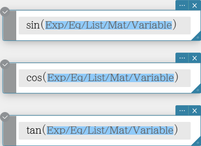
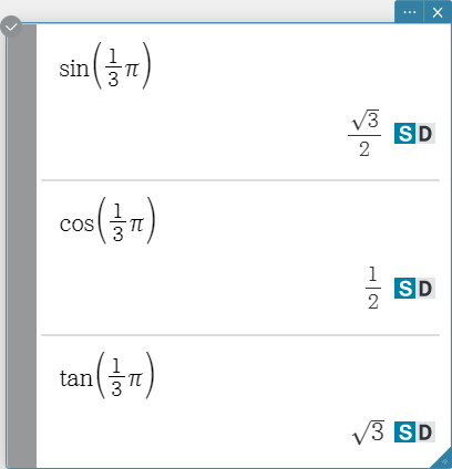
Trigonometric and Inverse Trigonometric Functions

sin, cos, tan

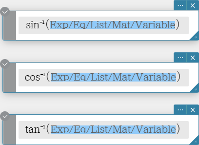
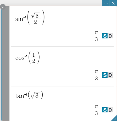
sin$ ^{- 1}$, cos$ ^{- 1}$, tan$ ^{- 1}$

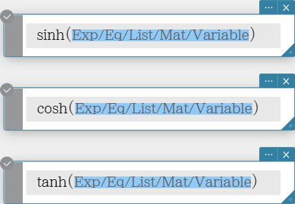
Hyperbolic and Inverse Hyperbolic Functions

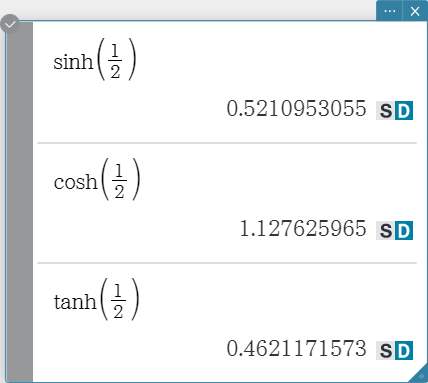
sinh, cosh, tanh

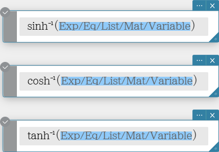
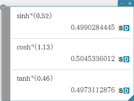
sinh$ ^{- 1}$, cosh$ ^{- 1}$, tanh$ ^{- 1}$

Angle Units

°　　　r

Mixed Fraction

mixedFraction
Syntax: $ ■\frac □□ $

Logarithmic Function

ln, log

Numeric Calculations

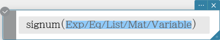
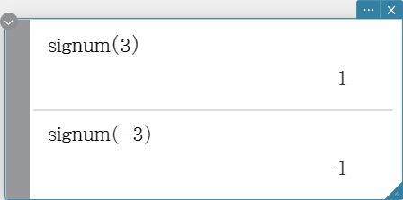
signum

signum returns –1 for a negative value, 1 for a positive value,
“Undefined” for 0, and $ \frac{A}{|A|} $ for an imaginary number.

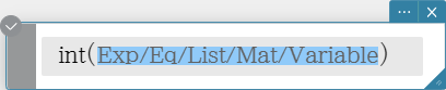
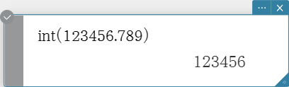
Int

Returns the integer part of a value.

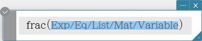
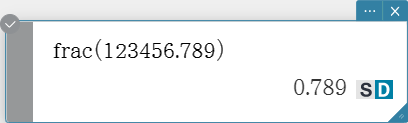
frac

Returns the decimal part of a value.

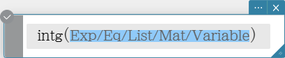
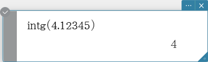
intg

Returns the largest integer that does not exceed a value.

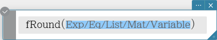
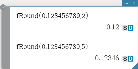
fRound

Rounds the decimal part of a value to the specified number of decimal places.
Syntax: fRound (Exp/Eq/List/Mat/Variable [ ) ]

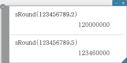
sRound

Rounds a value to the specified number of digits.
Syntax: sRound (Exp/Eq/List/Mat/Variable [ ) ]

Random Number Generator

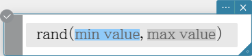
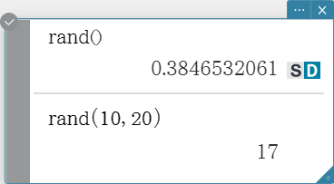
rand

Syntax: rand([a, b])

The “rand” function generates random numbers. If you do not specify an argument,
“rand” generates 10-digit decimal values 0 or greater and less than 1.

Specifying two integer values for the argument generates random numbers between them.

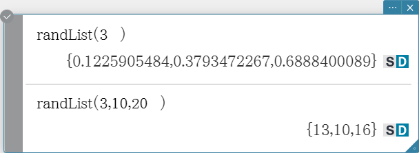
randList

Syntax: randList( n [, a, b])

Omitting arguments “a” and “b” returns a list of n elements that contain decimal random values.
Specifying arguments “a” and “b” returns a list of n elements that contain integer random values in the range of “a” through “b”.
“n” must be a positive integer.
The random numbers of each element are generated in accordance with “RandSeed” specifications.

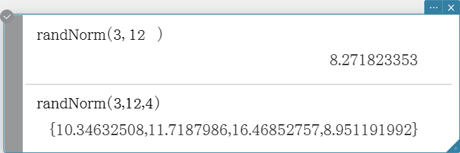
randNorm

The “randNorm” function generates a 10-digit normal random number based on a specified mean μ and standard deviation σ values.

Syntax: randNorm(σ, μ [, n ])

Omitting a value for “n” (or specifying 1 for “ n ”) returns the generated random number as-is.
Specifying 2 or larger value for “n” returns the specified number of random values in list format.
“n” must be a positive integer, and “σ” must be greater than 0.

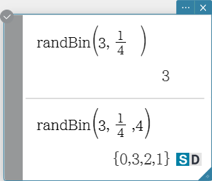
randBin

The “randBin” function generates binomial random numbers based on values specified for the number of trials n and probability P.
Syntax: randBin( n, P [, m ])

Omitting a value for “m” (or specifying 1 for “m”) returns the generated random number as-is.
Specifying a 2 or larger value for “m” returns the specified number of random values in list format.
“n” and “m” must be positive integers.

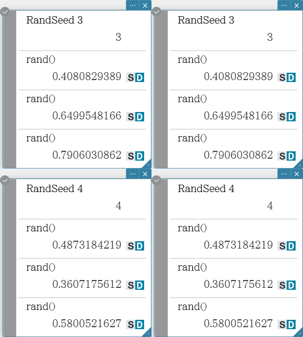
RandSeed

You can specify an integer from 0 to 9 for the argument of this command.
0 specifies non-sequential random number generation.
An integer from 1 to 9 uses the specified value as a seed for specification of sequential random numbers.
The initial default argument for this command is 0.
The numbers generated by the application immediately after you specify sequential random number generation always follow the same random pattern.

Integer Functions

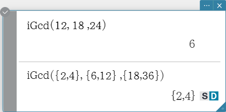
iGcd

Syntax: iGcd(Exp-1, Exp-2[, Exp-3…Exp-10)]
(Exp-1 through Exp-10 all are integers.)
iGcd(List-1, List-2[, List-3…List-10)]
(All elements of List-1 through List-10 are integers.)

The first syntax above returns the greatest common divisor for two to ten integers.
The second syntax returns, in list format, the greatest common divisor (GCD) for each
of the elements in two to ten lists. When the arguments are {a, b}, {c, d}, for example,
a list will be returned showing the GCD for a and c, and for b and d.

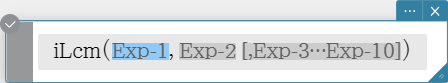
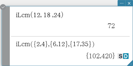
iLcm

Syntax: iLcm(Exp-1, Exp-2[, Exp-3…Exp-10)]
(Exp-1 through Exp-10 all are integers.)
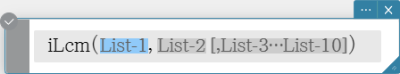
iLcm(List-1, List-2[, List-3…List-10)]
(All elements of List-1 through List-10 are integers.)

The first syntax above returns the least common multiple for two to ten integers.
The second syntax returns, in list format, the least common multiple (LCM) for each
of the elements in two to ten lists. When the arguments are {a, b}, {c, d}, for example,
a list will be returned showing the LCM for a and c, and for b and d.

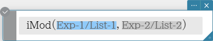
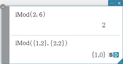
iMod

Syntax: iMod(Exp-1/List-1, Exp-2/List-2[)]
(Exp-1, Exp-2 and all of the elements of List-1 and List-2 must be integers.)

This function divides one or more integers by one or more other integers and returns the remainder(s).

Permutation and Combination

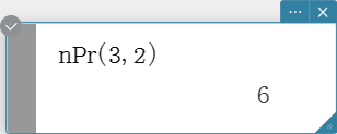
nPr

Syntax: nPr(n, r[)]
（“n” and “r” must be positive integers.）

Returns the total number of permutations where n is the total number of objects in the set and r is the number of objects chosen from the set.
\[ {}_n P_r = \frac{n!}{(n-r)!} \]

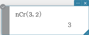
nCr

Syntax: nCr(n, r[)]
（“n” and “r” must be positive integers.）

Returns the total number of combinations where n is the total number of objects in the set and r is the number of objects chosen from the set.
\[ {}_n C_r = \frac{n!}{r!(n-r)!} \]

Other Functions

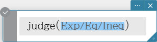
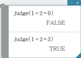
judge

The “judge” function returns TRUE when an expression is true, and FALSE when it is false.

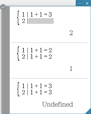
piecewise

The “piecewise” function returns one value when an expression is true,
and another value when the expression is false.

Syntax:

\[ \begin{cases} \lt \text{return value when true} \gt | \lt \text{condition expression} \gt \\
\lt \text{return value when false or indeterminate} \gt \end{cases} \]

or

\[ \begin{cases} \lt \text{return value when condition 1 is true} \gt | \lt \text{condition 1 expression}
\gt \\ \lt \text{return value when condition 2 is true} \gt | \lt \text{condition 2 expression}
\gt \end{cases} \]

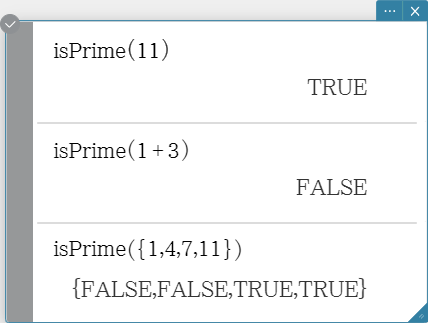
isPrime

The “isPrime” function determines whether the number provided as the argument is prime
(returns TRUE) or not (returns FALSE).

Syntax: isPrime(Exp/List[ ) ]

Exp or all of the elements of List must be integers.

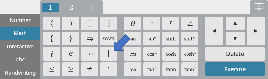
with Operator ( | )

The “with” ( | ) operator temporarily assigns a value to a variable.
You can use the “with” operator in the following cases.

To assign the value specified on the right side of | to the variable on the left side of |
To limit or restrict the range of a variable on the left side of | in accordance with
conditions provided on the right side of |

Syntax: Exp/Eq/Ineq/List/Mat | Eq/Ineq/List/(and operator)

You can put plural conditions in a list or connected with the “and” operator on the right side.
“$\small{\neq}$” can be used on the left side or the right side of |.

Note

Use the [Math] keyboard to input |.

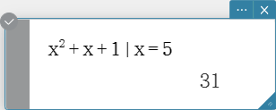
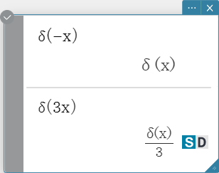
delta

“delta” is the Dirac Delta function. The delta function evaluates numerically as shown below.

\[ \delta(x) = \begin{cases} 0, x \neq 0 \\ \delta(x), x=0 \end{cases} \]
$ x $ : variable or number

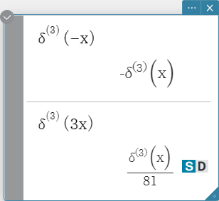
$n$th-delta

The $n$th-delta function is the $n$th differential of the delta function.
Syntax: $ δ^{(n)} (x) $
$ x $ : variable or number
$ n $ : number of differentials

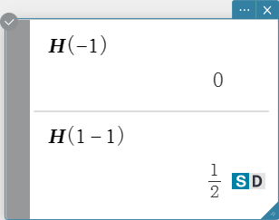
heaviside

“heaviside” is the command for the Heaviside function, which evaluates only to numeric expressions as shown below.
\[ H(x) = \begin{cases} 0, x<0 \\ \frac 12, x = 0 \\ 1, x>0 \end{cases} \]
$ x $ : variable or number

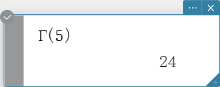
gamma

“gamma” is the command for the Gamma function.
Syntax: $ \Gamma (x) = \int_0^{+\infty} t^{x-1} e^{-t} dt $
$ x $ : variable or number

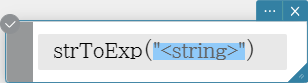
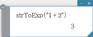
strToExp

Converts a string to an expression, and executes the expression.
Syntax: strToExp («<string>»)

Transformation

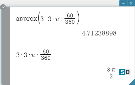
approx

Transforms an expression into a numerical approximation.
Syntax: approx (Exp/Eq/List/Mat/Variable [ ) ]

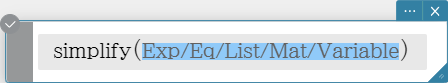
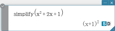
simplify

Simplifies an expression.
Syntax: simplify (Exp/Eq/List/Mat/Variable [ ) ]

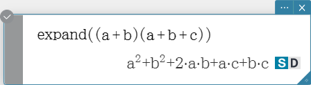
expand

Expands an expression.
Syntax: expand (Exp/Eq/List/Mat/Variable [ ) ]
expand (Exp,Variable [ ) ]

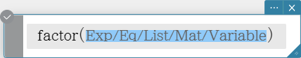
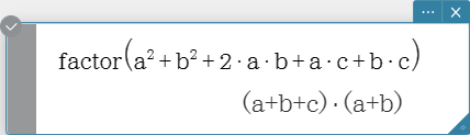
factor

Factors an expression.
Syntax: factor (Exp/Eq/List/Mat/Variable [ ) ]

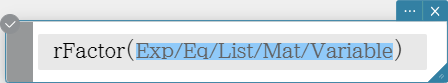
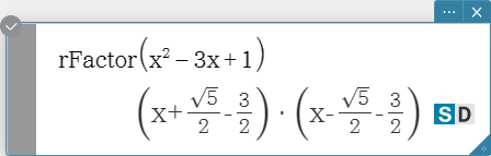
rFactor

Factors an expression up to its roots, if any.
Syntax: rFactor (Exp/Eq/List/Mat/Variable [ ) ] ]

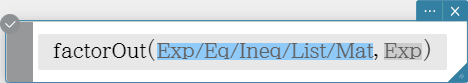
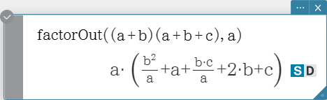
factorOut

Factors out an expression with respect to a specified factor.
Syntax: factorOut (Exp/Eq/Ineq/List/Mat, Exp [ ) ]

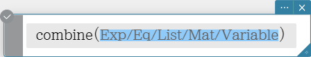
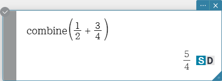
combine

Transforms multiple fractions into their common denominator equivalents and reduces them, if possible.
Syntax: combine (Exp/Eq/List/Mat/Variable [ ) ]

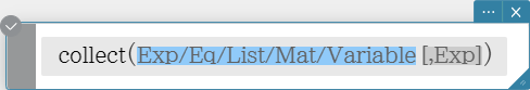
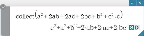
collect

Rearranges an expression with respect to a specific variable.
Syntax: collect (Exp/Eq/List/Mat/Variable[, Exp] [ ) ]

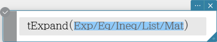
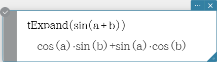
tExpand

Employs the sum and difference formulas to expand a trigonometric function.
Syntax: tExpand (Exp/Eq/Ineq/List/Mat [ ) ]

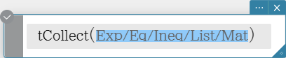
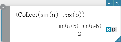
tCollect

Employs the product to sum formulas to transform the product of a trigonometric
function into an expression in the sum form.

Syntax: tCollect (Exp/Eq/Ineq/List/Mat [ ) ]

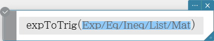
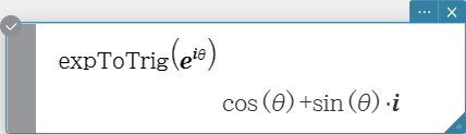
expToTrig

Transforms an exponent into a trigonometric or hyperbolic function.
Syntax: expToTrig (Exp/Eq/Ineq/List/Mat [ ) ]

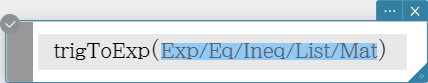
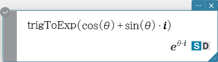
trigToExp

Transforms a trigonometric or hyperbolic function into exponential form.
Syntax: trigToExp (Exp/Eq/Ineq/List/Mat [ ) ]

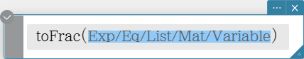
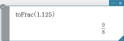
toFrac

Transforms a decimal value into its equivalent fraction value.
Syntax: toFrac (Exp/Eq/List/Mat/Variable [ ) ]

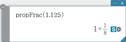
propFrac

Transforms a decimal value into its equivalent proper fraction value.
Syntax: propFrac (Exp/Eq/Ineq/List/Mat [ ) ]

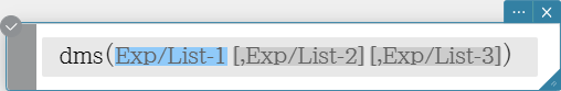
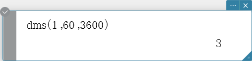
dms

Transforms a DMS format value into its equivalent degrees-only value.
Syntax: dms (Exp/List-1 [, Exp/List-2][, Exp/List-3] [ ) ]

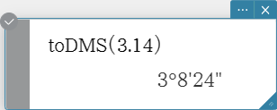
toDMS

Transforms a degrees-only value into its equivalent DMS format value.
Syntax: toDMS (Exp/List [ ) ]

Advanced

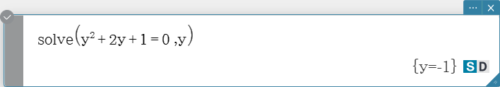
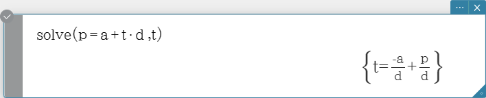
solve

Returns the solution of an equation or inequality.
Syntax 1: solve(Exp/Eq/Ineq [, Variable] [ ) ]

“$x$” is the default when you omit “[, Variable]”.

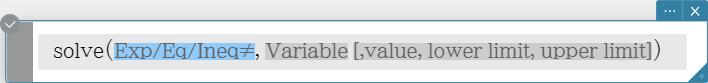
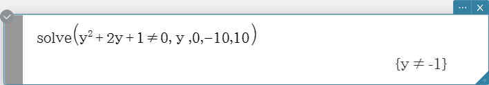
Syntax 2: solve(Exp/Eq/Ineq$\small{\neq}$, Variable[, value, lower limit, upper limit] [ ) ]

“value” is an initially estimated value.
This command is valid only for equations and $\small{\neq}$ expressions when “value” and the items
following it are included. In that case, this command returns an approximate value.
A true value is returned when you omit “value” and the items following it.
When, however, a true value cannot be obtained, an approximate value is returned for
equations only based on the assumption that value = 0, lower limit = – ∞, and upper limit = ∞.

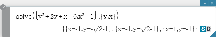
Syntax 3: solve({Exp-1/Eq-1, …, Exp-N/Eq-N}, {variable-1, …, variable-N} [ ) ]

When “Exp” is the first argument, the equation Exp = 0 is presumed.

Syntax 4: You can solve for the relationship between two points, straight lines, planes, or
spheres by entering a vector equation inside the solve( command. Here we will
present four typical syntaxes for solving a vector equation using the solve( command.

In the syntaxes below, Vct-1 through Vct-6 are column vectors with three (or two) elements, and s, t, u and
v are parameters.

solve(Vct-1 + s * Vct-2 [= Vct-3, {variable-1}])

If the right side of the equation (= Vct-3) is omitted in the above syntax,
it is assumed that all of the elements on the right side are 0 vectors.

solve(Vct-1 + s * Vct-2 = Vct-3 + t * Vct-4, {variable-1, variable-2})
solve(Vct-1 + s * Vct-2 + t * Vct-3 = Vct-4 – u * Vct-5, {variable-1, variable-2, variable-3})
solve(Vct-1 + s * Vct-2 + t * Vct-3 = Vct-4 – u * Vct-5 + v * Vct-6, {variable-1, variable-2, variable-3, variable-4})

Variables (variable 1 through variable 4) can be input into the elements of each vector
(Vct-1 through Vct-6) in the above four syntaxes to solve for those variables.

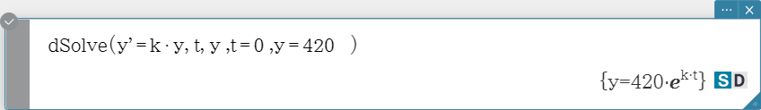
dSolve

Solves first, second or third order ordinary differential equations, or a system of first order differential equations.
Syntax: dSolve(Eq, independent variable, dependent variable [, initial condition-1, initial condition-2][, initial condition-3, initial condition-4][, initial condition-5, initial condition-6] [ ) ]
dSolve({Eq-1, Eq-2}, independent variable, {dependent variable-1, dependent variable-2} [, initial condition-1, initial condition-2, initial condition-3, initial condition-4] [ ) ]

If you omit the initial conditions, the solution will include arbitrary constants.
Input all initial conditions equations using the syntax Var = Exp. Any initial condition that uses any other syntax will be ignored.

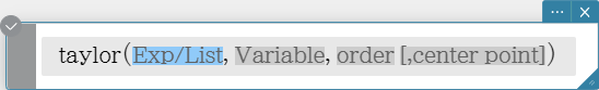
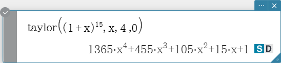
taylor

Finds a Taylor polynomial for an expression with respect to a specific variable.
Syntax: taylor (Exp/List, Variable, order [, center point] [ ) ]

Zero is the default when you omit “[, center point]”.

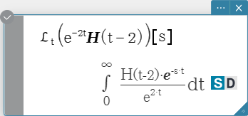
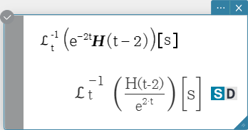
laplace, invLaplace

“laplace” is the command for the Laplace transform, and “invLaplace” is the command for
the inverse of Laplace transform.

Syntax: laplace $ ℒ_t (f(t))[s] $
$ f(t) $: expression
$ t $: variable with respect to which the expression is transformed
$ s $: parameter of the transform
invLaplace $ ℒ_s^{-1} (L(s))[t] $
$ L(s) $: expression
$ s $: variable with respect to which the expression is transformed
$ t $: parameter of the transform

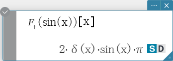
fourier, invFourier

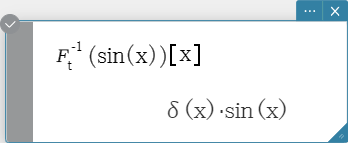
“fourier” is the command for the Fourier Transform, and “invFourier” is
the command for the inverse Fourier Transform.

Syntax: fourier $Ϝ_x (f(x))[w] $
invFourier $ Ϝ_w^{-1} (f(w))[x] $
$ x $: variable with respect to which the expression is transformed
$ w $: parameter of the transform

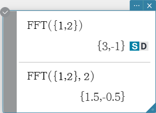
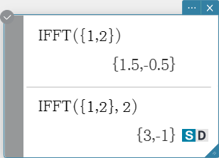
FFT, IFFT

“FFT” is the command for the fast Fourier Transform, and “IFFT” is the command for the inverse fast Fourier Transform.
2n data values are needed to perform FFT and IFFT. FFT and IFFT are calculated numerically.

Syntax: FFT(list) or FFT(list, m )
IFFT(list) or IFFT(list, m )

Data size must be 2n for n = 1, 2, 3, …
The value for m is optional. It can be from 0 to 2, indicating the FFT parameter to use:
0 (Signal Processing), 1 (Pure Math), 2 (Data Analysis).

Calculation

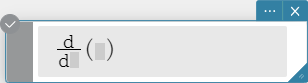
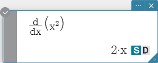
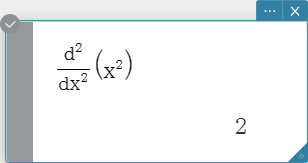
diff

Differentiates an expression with respect to a specific variable.

Syntax:
$ \frac{\mathrm d}{\mathrm d ■} □ $,
$ \frac{\mathrm d^□}{\mathrm d ■} □ $

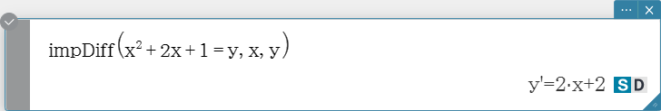
impDiff

Differentiates an equation or expression in implicit form with respect to a specific variable.

Syntax: impDiff(Eq/Exp/List, independent variable, dependent variable)

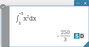
Integrate

Integrates an expression with respect to a specific variable.
Syntax: $ \int_□^□ ■ d□ $

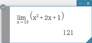
lim

Determines the limit of an expression.
Syntax: $$ \lim_{■ \to □} (■)$$

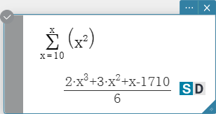
sum

Evaluates an expression at discrete variable values within a range, and then calculates a sum.
Syntax: $ \sum_{■=□}^{□} (⬚) $

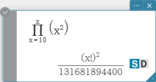
prod

Evaluates an expression at discrete variable values within a range, and then calculates a product.
Syntax: $ \prod_{■=□}^{□} ■ $

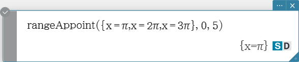
rangeAppoint

Finds an expression or value that satisfies a condition in a specified range.
Syntax: rangeAppoint (Exp/Eq/List, start value, end value [ ) ]

When using an equation (Eq) for the first argument, input the equation using the syntax Var
= Exp. Evaluation will not be possible if any other syntax is used.

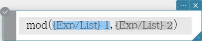
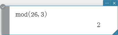
mod

Returns the remainder when one expression is divided by another expression.
Syntax: mod ({Exp/List} -1, {Exp/List} -2 [ ) ]

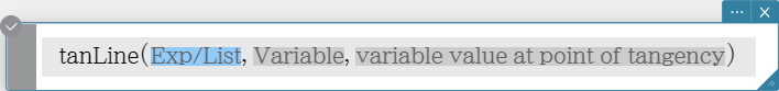
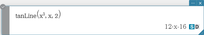
tanLine

Returns the right side of the equation for the tangent line (y = ‘expression’) to the curve at the specified point.
Syntax: tanLine (Exp/List, Variable, variable value at point of tangency [ ) ]

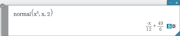
normal

Returns the right side of the equation for the line normal (y = ‘expression’)
to the curve at the specified point.

Syntax: normal (Exp/List, Variable, variable value at point of normal [ ) ]

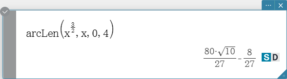
arcLen

Returns the arc length of an expression from a start value to an end value
with respect to a specified variable.

Syntax: arcLen (Exp/List, Variable, start value, end value [ ) ]

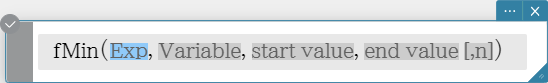
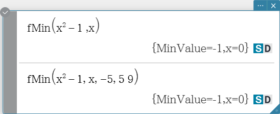
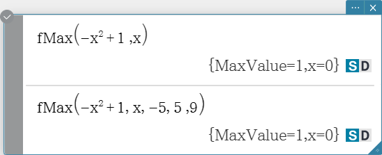
fMin, fMax

Returns the minimum (fMin) / the maximum (fMax) point in a specific range of a function.

Syntax: fMin(Exp[, Variable] [ ) ]
fMin(Exp, Variable, start value, end value[, n] [ ) ]
fMax(Exp[, Variable] [ ) ]
fMax(Exp, Variable, start value, end value[, n] [ ) ]

“x” is the default when you omit “[, Variable]”.
Negative infinity and positive infinity are the default when the syntax
fMin(Exp[, Variable] [ ) ] or fMax(Exp[, Variable] [ ) ] is used.
“n” is calculation precision, which you can specify as an integer in the
range of 1 to 9. Using any value outside this range causes an error.
This command returns an approximate value when calculation precision is specified for “n”.
This command returns a true value when nothing is specified for “n”. If the true value cannot
be obtained, however, this command returns an approximate value along with n = 4.
Discontinuous points or sections that fluctuate widely can adversely affect
precision or even cause an error.
Inputting a larger number for “n” increases the precision of the calculation,
but it also increases the amount of time required to perform the calculation.
The value you input for the end point of the interval must be greater than the
value you input for the start point. Otherwise an error occurs.

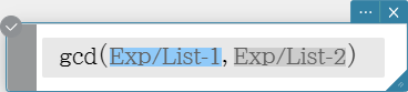
gcd

Returns the greatest common denominator of two expressions.

Syntax: gcd (Exp/List-1, Exp/List-2 [ ) ]

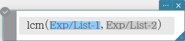
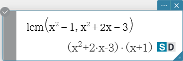
lcm

Returns the least common multiple of two expressions.
Syntax: lcm (Exp/List-1, Exp/List-2 [ ) ]

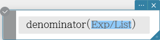
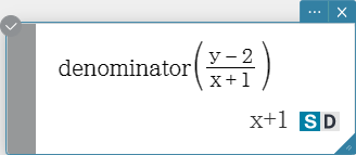
denominator

Extracts the denominator of a fraction.
Syntax: denominator (Exp/List [ ) ]

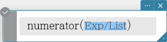
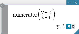
numerator

Extracts the numerator of a fraction.
Syntax: numerator (Exp/List [ ) ]

Complex

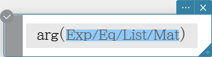
arg

Returns the argument of a complex number.
Syntax: arg (Exp/Eq/List/Mat [ ) ]

conjg

Returns the conjugate complex number.
Syntax: conjg (Exp/Eq/Ineq$\small{\neq}$/List/Mat [ ) ] (Ineq$\small{\neq}$: Real mode only)

re

Returns the real part of a complex number.
Syntax: re (Exp/Eq/Ineq$\small{\neq}$/List/Mat [ ) ] (Ineq$\small{\neq}$: Real mode only)

im

Returns the imaginary part of a complex number.
Syntax: im (Exp/Eq/Ineq$\small{\neq}$/List/Mat [ ) ] (Ineq$\small{\neq}$: Real mode only)

cExpand

Expands a complex expression to rectangular form (a + bi).
Syntax: cExpand (Exp/Eq/List/Mat [ ) ]

The variables are regarded as real numbers.

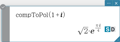
compToPol

Transforms a complex number into its polar form.
Syntax: compToPol (Exp/Eq/List/Mat [ ) ]

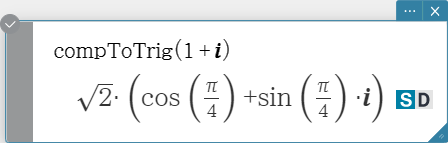
compToTrig

Transforms a complex number into its trigonometric/hyperbolic form.
Syntax: compToTrig (Exp/Eq/List/Mat [ ) ]

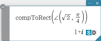
compToRect

Transforms a complex number into its rectangular form.
Syntax: compToRect ($∠(r, \theta)$ or $r \cdot e$^$(\theta \cdot i)$ form [ ) ]

List

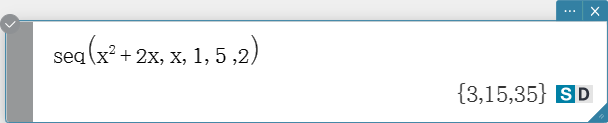
seq

Generates a list in accordance with a numeric sequence expression.
Syntax: seq (Exp, Variable, start value, end value [, step size] [ ) ]

“1” is the default when you omit “[, step size]”.
The step size must be a factor of the difference between the start value and the end value.

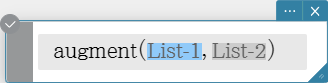
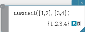
augment

Creates a new list by appending one list to another.
Syntax: augment (List-1, List-2 [ ) ]

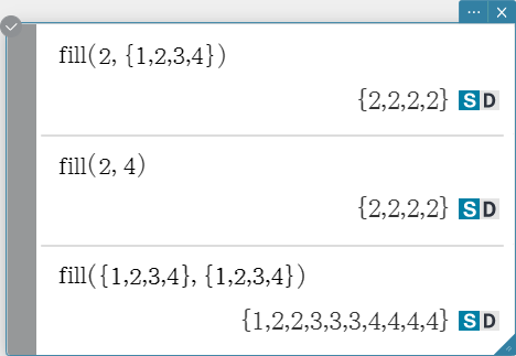
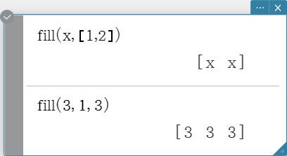
fill

Replaces the elements of a list with a specified value or expression. This command can also beused to create a new list whose elements all contain the same value or expression, or a new list inwhich the frequency of each element in the first list is determined by the corresponding element inthe second list.
Syntax: fill (Exp/Eq/Ineq, number of elements [ ) ]
fill (Exp/Eq/Ineq, List [ ) ]
fill (List, List [ ) ]

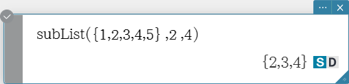
subList

Extracts a specific section of a list into a new list.
Syntax: subList (List [, start number] [, end number] [ ) ]

The leftmost element is the default when you omit “[, start number]”, and the rightmost element is the default when you omit “[, end number]”.

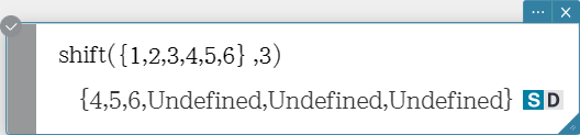
shift

Returns a list in which elements have been shifted to the right or left by a specific amount.
Syntax: shift (List [, number of shifts] [ ) ]

Specifying a negative value for “[, number of shifts]” shifts to the right, while a positive value shifts to the left.
Right shift by one (–1) is the default when you omit “[, number of shifts]”.

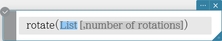
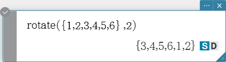
rotate

Returns a list in which the elements have been rotated to the right or to the left by a specific amount.
Syntax: rotate (List [, number of rotations] [ ) ]

Specifying a negative value for “[, number of rotations]” rotates to the right, while a positive value rotates to the left.
Right rotation by one (–1) is the default when you omit “[, number of rotations]”.

sortA

Sorts the elements of the list into ascending order.
Syntax: sortA (List [ ) ]

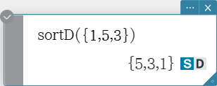
sortD

Sorts the elements of the list into descending order.
Syntax: sortD (List [ ) ]

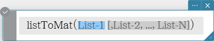
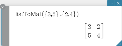
listToMat

Transforms lists into a matrix.
Syntax: listToMat (List-1 [, List-2, …, List-N] [ ) ]

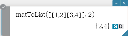
matToList

Transforms a specific column of a matrix into a list.
Syntax: matToList (Mat, column number [ ) ]

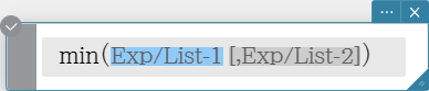
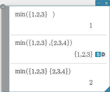
min

Returns the minimum value of an expression or the elements in a list.
Syntax: min (Exp/List-1[, Exp/List-2] [ ) ]

max

Returns the maximum value of an expression or the elements of a list.
Syntax: max (Exp/List-1[, Exp/List-2] [ ) ]

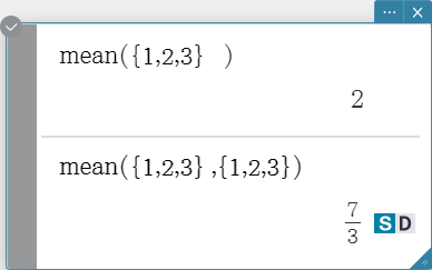
mean

Returns the mean of the elements in a list.
Syntax: mean (List-1[, List-2] [ ) ] (List-1: Data, List-2: Freq)

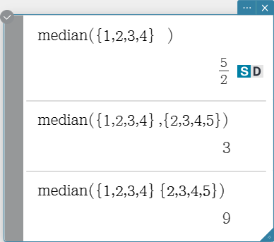
median

Returns the median of the elements in a list.
Syntax: median (List-1[, List-2] [ ) ] (List-1: Data, List-2: Freq)

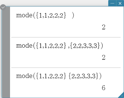
mode

Returns the mode of the elements in a list. If there are multiple modes, they are returned in a list.
Syntax: mode (List-1[, List-2] [ ) ] (List-1: Data, List-2: Freq)

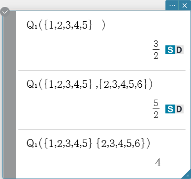
$ Q_1 $

Returns the first quartile of the elements in a list.
Syntax: $ Q_1 $ (List-1[, List-2] [ ) ] (List-1: Data, List-2: Freq)

$ Q_3 $

Returns the third quartile of the elements in a list.
Syntax: $ Q_3 $ (List-1[, List-2] [ ) ] (List-1: Data, List-2: Freq)

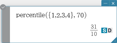
percentile

Finds the $n$ th percentile point in a list.
Syntax: percentile (List, number)

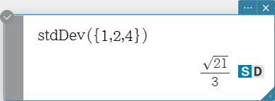
stdDev

Returns the sample standard deviation of the elements in a list.
Syntax: stdDev (List [ ) ]

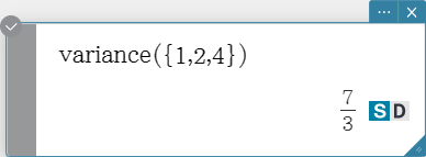
variance

Returns the sample variance of the elements in a list.
Syntax: variance (List [ ) ]

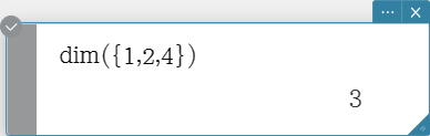
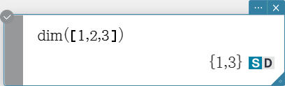
dim

Returns the dimension of a list.
Syntax: dim (List [ ) ]

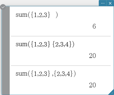
sum

Returns the sum of the elements in a list.
Syntax: sum (List-1[, List-2] [ ) ] (List-1: Data, List-2: Freq)

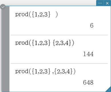
prod

Returns the product of the elements in a list.
Syntax: prod (List-1[, List-2] [ ) ] (List-1: Data, List-2: Freq)

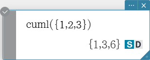
cuml

Returns the cumulative sums of the elements in a list.
Syntax: cuml (List [ ) ]

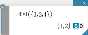
⊿list

Returns a list whose elements are the differences between two adjacent elements in another list.
Syntax: ⊿list (List [ ) ]

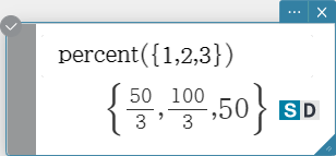
percent

Returns the percentage of each element in a list, the sum of which is assumed to be 100.
Syntax: percent (List [ ) ]

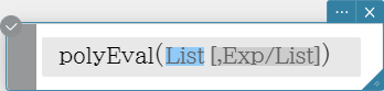
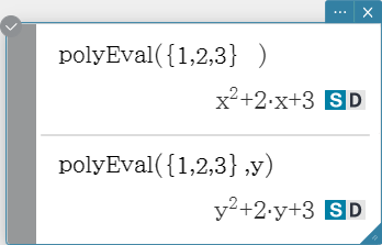
polyEval

Returns a polynomial arranged in the descending order of powers, so coefficients correspond sequentially to each element in the input list.
Syntax: polyEval (List [, Exp/List] [ ) ]

“$x$” is the default when you omit “[, Exp/List]”.

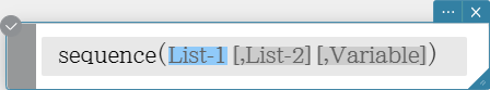
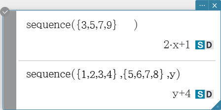
sequence

Returns the lowest-degree polynomial that represents the sequence expressed by the input list. When there are two lists, this command returns a polynomial that maps each element in the first list to its corresponding element in the second list.
Syntax: sequence (List-1[, List-2] [, Variable] [ ) ]

“$x$” is the default when you omit “[, Variable]”.

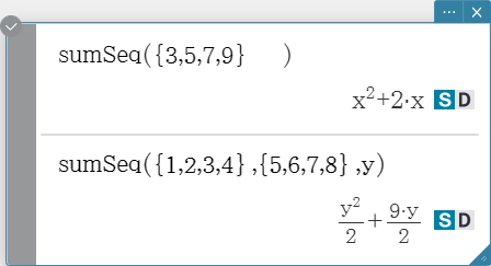
sumSeq

Finds the lowest-degree polynomial that represents the sequence expressed by the input list and returns the sum of the polynomial. When there are two lists, this command returns a polynomial that maps each element in the first list to its corresponding element in the second list, and returns the sum of the polynomial.
Syntax: sumSeq (List-1[, List-2] [, Variable] [ ) ]

“$x$” is the default when you omit “[, Variable]”.

Matrix

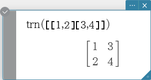
trn

Returns a transposed matrix.
Syntax: trn (Mat [ ) ]

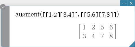
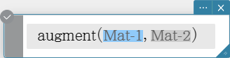
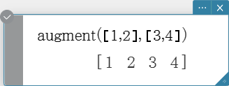
augment

Returns a matrix that combines two other matrices.
Syntax: augment (Mat-1, Mat-2 [ ) ]

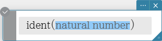
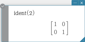
ident

Creates an identity matrix.
Syntax: ident (natural number [ ) ]

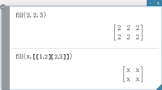
fill

Creates a matrix with a specific number of rows and columns, or replaces the elements of a matrix with a specific expression.
Syntax: fill (Exp, number of rows, number of columns [ ) ]
fill (Exp, Mat [ ) ]

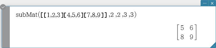
subMat

Extracts a specific section of a matrix into a new matrix.
Syntax: subMat (Mat [, start row] [, start column] [, end row] [, end column] [ ) ]

“1” is the default when you omit “[, start row]” and “[, start column]”.
The last row number is the default when you omit “[, end row]”.
The last column number is the default when you omit “[, end column]”.

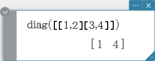
diag

Returns a one-row matrix containing the elements from the main diagonal of a square matrix.
Syntax: diag (Mat[ ) ]

listToMat

Transforms lists into a matrix.
Syntax: listToMat (List-1 [, List-2, …, List-N] [ ) ]

matToList

Transforms a specific column of a matrix into a list.
Syntax: matToList (Mat, column number [ ) ]

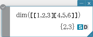
dim

Returns the dimensions of a matrix as a two-element list {number of rows, number of columns}.
Syntax: dim (Mat [ ) ]

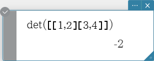
det

Returns the determinant of a square matrix.
Syntax: det (Mat [ ) ]

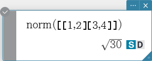
norm

Returns the Frobenius norm of the matrix.
Syntax: norm (Mat [ ) ]

rank

Finds the rank of matrix.
The rank function computes the rank of a matrix by performing Gaussian elimination on the rows of the given matrix. The rank of matrix A is the number of non-zero rows in the resulting matrix.
Syntax: rank (Mat [ ) ]

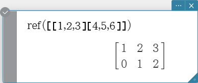
ref

Returns the row echelon form of a matrix.
Syntax: ref (Mat [ ) ]

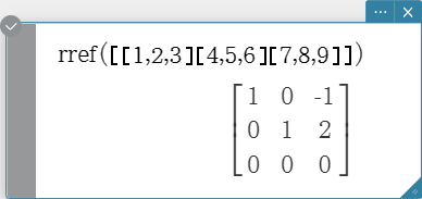
rref

Returns the reduced row echelon form of a matrix.
Syntax: rref (Mat [ ) ]

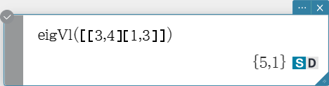
eigVl

Returns a list that contains the eigenvalue(s) of a square matrix.
Syntax: eigVl (Mat [ ) ]

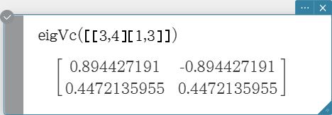
eigVc

Returns a matrix in which each column represents an eigenvector of a square matrix.

Since an eigenvector usually cannot be determined uniquely, it is standardized as follows to its norm, which is 1:

When ${\rm V} = [ x_1, x_2, …, x_n ]$, $\sqrt{\left( |x_1|^2+|x_2|^2+…+|x_n|^2 \right)}=1$.
Syntax: eigVc (Mat [ ) ]

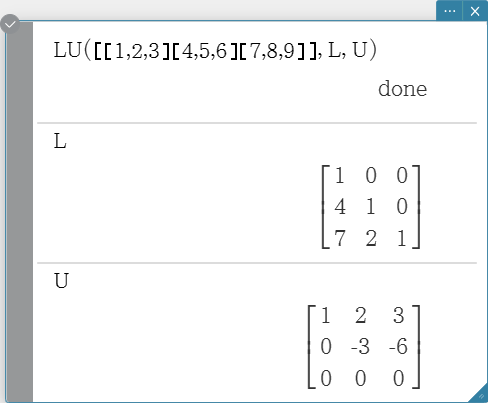
LU

Returns the LU decomposition of a square matrix.
Syntax: LU (Mat, lVariableMem, uVariableMem [ ) ]

The lower matrix is assigned to the first variable L, while the upper matrix is assigned to the second variable U.

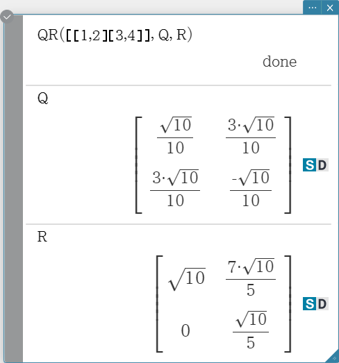
QR

Returns the QR decomposition of a square matrix.
Syntax: QR (Mat, qVariableMem, rVariableMem [ ) ]
Example: To obtain the QR decomposition of the matrix [[1, 2] [3, 4]]

The unitary matrix is assigned to variable Q, while the upper triangular matrix is assigned to variable R.

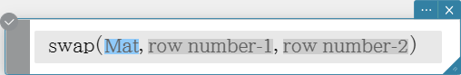
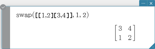
swap

Swaps two rows of a matrix.
Syntax: swap (Mat, row number-1, row number-2 [ ) ]

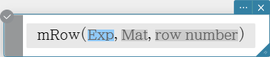
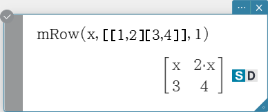
mRow

Multiplies the elements of a specific row in a matrix by a specific expression.
Syntax: mRow (Exp, Mat, row number [ ) ]

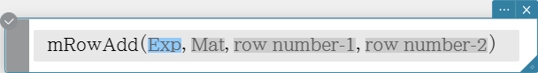
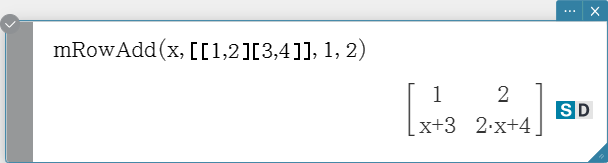
mRowAdd

Multiplies the elements of a specific row in a matrix by a specific expression, and then adds the result to another row.
Syntax: mRowAdd (Exp, Mat, row number-1, row number-2 [ ) ]

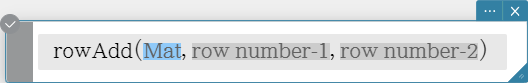
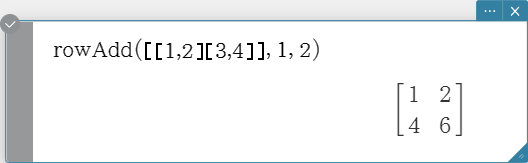
rowAdd

Adds a specific matrix row to another row.
Syntax: rowAdd (Mat, row number-1, row number-2 [ ) ]

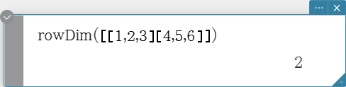
rowDim

Returns the number in rows in a matrix.
Syntax: rowDim (Mat [ ) ]

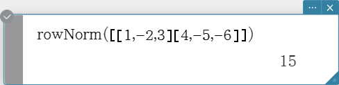
rowNorm

Calculates the sums of the absolute values of the elements of each row of a matrix, and returns the maximum value of the sums.
Syntax: rowNorm (Mat [ ) ]

colDim

Returns the number of columns in a matrix.
Syntax: colDim (Mat [ ) ]

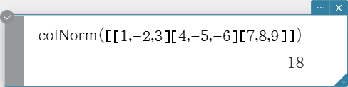
colNorm

Calculates the sums of the absolute values of the elements of each column of a matrix, and returns the maximum value of the sums.
Syntax: colNorm (Mat [ ) ]

Vector

A vector is handled as a 1 $\times$ N matrix or N $\times$ 1 matrix.
A vector in the form of 1 $\times$ N can be entered as [……] or [[……]].
Example: [1, 2], [[1, 2]]
Vectors are considered to be in rectangular form unless ∠() is used to indicate an angle measure.

augment

Returns an augmented vector [Mat-1 Mat-2].
Syntax: augment (Mat-1, Mat-2 [ ) ]

fill

Creates a vector that contains a specific number of elements, or replaces the elements of a vector with a specific expression.
Syntax: fill (Exp, Mat [ ) ]
fill (Exp, 1, number of columns [ ) ]

dim

Returns the dimension of a vector.
Syntax: dim (Mat [ ) ]

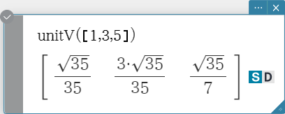
unitV

Normalizes a vector.
Syntax: unitV (Mat [ ) ]

This command can be used with a 1 $\times$ N or N $\times$ 1 matrix only.

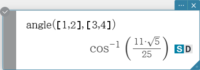
angle

Returns the angle formed by two vectors.
Syntax: angle (Mat-1, Mat-2 [ ) ]

This command can be used with a 1 $\times$ N or N $\times$ 1 matrix only.

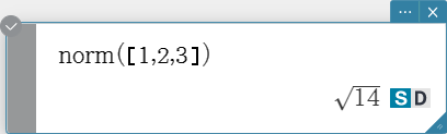
norm

Returns the norm of a vector.
Syntax: norm (Mat [ ) ]

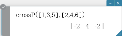
crossP

Returns the cross product of two vectors.
Syntax: crossP (Mat-1, Mat-2 [ ) ]

This command can be used with a 1 $\times$ N or N $\times$ 1 matrix only (N = 2, 3).
A two-element matrix [a, b] or [[a], [b]] is automatically converted into a three-element matrix [a, b, 0] or [[a], [b], [0]].

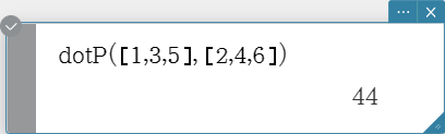
dotP

Returns the dot product of two vectors.
Syntax: dotP (Mat-1, Mat-2 [ ) ]

This command can be used with a 1 $\times$ N or N $\times$ 1 matrix only.

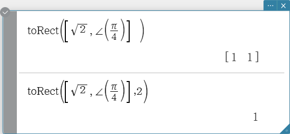
toRect

Returns an equivalent rectangular form $[\ x\ y\ ]$ or $[\ x\ y\ z\ ]$.
Syntax: toRect (Mat [, natural number] [ ) ]

This command can be used with a 1 $\times$ N or N $\times$ 1 matrix only (N = 2, 3).
This command returns “x” when “natural number” is 1, “y” when “natural number” is 2, and “z” when “natural number” is 3.
This command returns a rectangular form when you omit “natural number”.

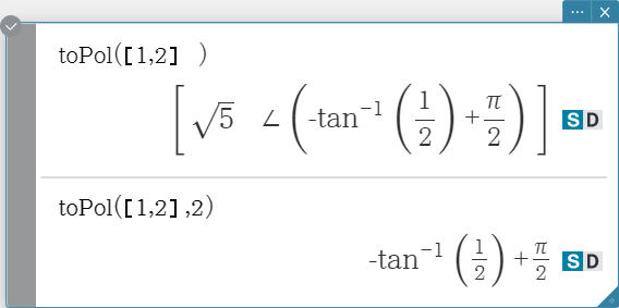
toPol

Returns an equivalent polar form $[\ r\ ∠\theta\ ]$.
Syntax: toPol (Mat [, natural number] [ ) ]

This command can be used with a 1 $\times$ 2 or 2 $\times$ 1 matrix only.
This command returns “$r$” when “natural number” is 1, and “$\theta$” when “natural number” is 2.
This command returns a polar form when you omit “natural number”.

toSph

Returns an equivalent spherical form $[\ \rho\ ∠\theta\ \ ∠\phi\ ]$.
Syntax: toSph (Mat [, natural number] [ ) ]

This command can be used with a 1 $\times$ 3 or 3 $\times$ 1 matrix only.
This command returns “$\rho$” when “natural number” is 1, “$\theta$” when “natural number” is 2, and “$\phi$” when “natural number” is 3.
This command returns a spherical form when you omit “natural number”.

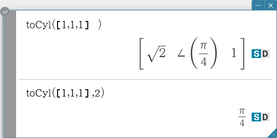
toCyl

Returns an equivalent cylindrical form $[\ r\ ∠\theta\ \ z\ ]$.
Syntax: toCyl (Mat [, natural number] [ ) ]

This command can be used with a 1 $\times$ 3 or 3 $\times$ 1 matrix only.
This command returns “$r$” when “natural number” is 1, “$\theta$” when “natural number” is 2, and “$z$” when “natural number” is 3.
This command returns a cylindrical form when you omit “natural number”.

Equation/Inequality

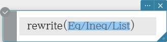
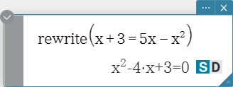
rewrite

Moves the right side elements of an equation or inequality to the left side.
Syntax: rewrite (Eq/Ineq/List [ ) ]

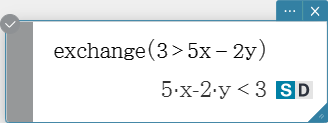
exchange

Swaps the right-side and left-side elements of an equation or inequality.
Syntax: exchange (Eq/Ineq/List [ ) ]

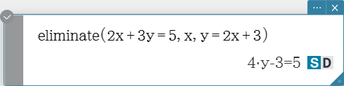
eliminate

Solves one equation with respect to a variable, and then replaces the same variable in another expression with the obtained result.
Syntax: eliminate (Eq/Ineq/List-1, Variable, Eq-2 [ ) ]

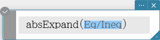
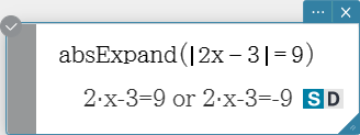
absExpand

Divides an absolute value expression into formulas without absolute value.
Syntax: absExpand (Eq/Ineq [ ) ]

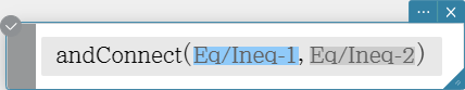
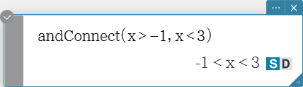
andConnect

Combines two equations or inequalities into a single expression.
Syntax: andConnect (Eq/Ineq-1, Eq/Ineq-2 [ ) ]

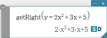
getRight

Extracts the right-side elements of an equation or inequality.
Syntax: getRight (Eq/Ineq/List [ ) ]

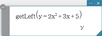
getLeft

Extracts the left-side elements of an equation or inequality.
Syntax: getLeft (Eq/Ineq/List [ ) ]

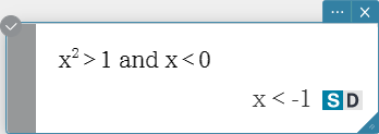
and

Returns the result of the logical AND of two expressions.
Syntax: Exp/Eq/Ineq/List-1 and Exp/Eq/Ineq/List-2

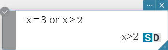
or

Returns the result of the logical OR of two expressions.
Syntax: Exp/Eq/Ineq/List-1 or Exp/Eq/Ineq/List-2

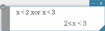
xor

Returns the logical exclusive OR of two expressions.
Syntax: Exp/Eq/Ineq/List-1 xor Exp/Eq/Ineq/List-2

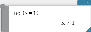
not

Returns the logical NOT of an expression.
Syntax: not(Exp/Eq/Ineq/List [ ) ]

Assistant

Note that the following commands are valid in the Assistant mode only. For more information on the Assistant mode see “2-14. Configuring Calculation Settings”.

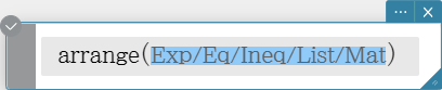
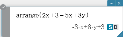
arrange

Combines common terms in an expression and returns the result arranged in descending sequence.
Syntax: arrange (Exp/Eq/Ineq/List/Mat [ ) ]

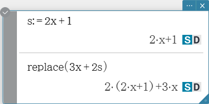
replace

Replaces the variable in an expression, equation or inequality with the value assigned to a variable using the “store” command.
Syntax: replace (Exp/Eq/Ineq/List/Mat [ ) ]

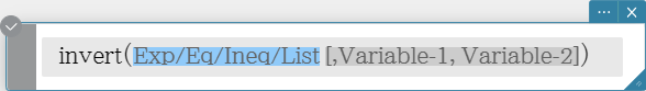
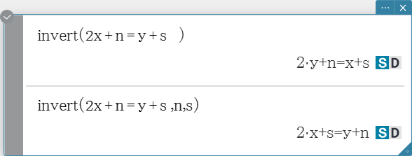
invert

Inverts two variables in an expression.
Syntax: invert (Exp/Eq/Ineq/List [, Variable-1, Variable-2] [ ) ]

x and y are inverted when variables are not specified.

Distribution/Inverse Distribution

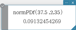
normPDf

Returns the normal probability density for a specified value.
Syntax: normPDf (x[, σ, μ)]

When σ and μ are skipped, σ = 1 and μ = 0 are used.

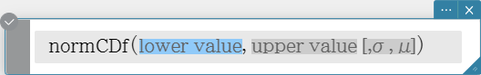
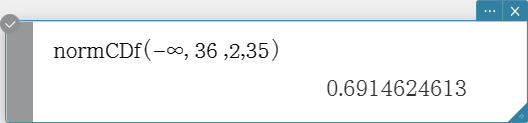
normCDf

Returns the cumulative probability of a normal distribution between a lower bound and an upper bound.
Syntax: normCDf (lower value, upper value[, σ, μ)]

When σ and μ are skipped, σ = 1 and μ = 0 are used.

Calculation Result Output: prob, zLow, zUp

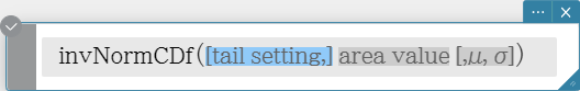
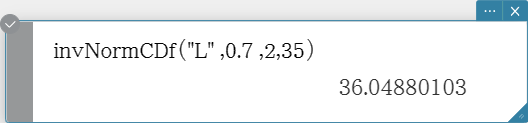
invNormCDf

Returns the boundary value(s) of a normal cumulative distribution probability for specified values.
Syntax: invNormCDf ([tail setting, ]area value[, σ, μ)]

When σ and μ are skipped, σ = 1 and μ = 0 are used.
“tail setting” displays the probability value tail specification, and Left, Right, or Center can be specified. Enter the following values or letters to specify:
Left: −1, “L”, or “l”
Center: 0, “C”, or “c”
Right: 1, “R”, or “r”

When input is skipped, “Left” is used.
When “tail setting” is Center, the lower bound value is returned.

Calculation Result Output: x₁InvN, x₂InvN

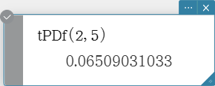
tPDf

Returns the Student’s t probability density for a specified value.
Syntax: tPDf (x, df [ ) ]
Calculation Result Output: prob

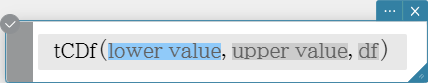
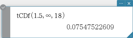
tCDf

Returns the cumulative probability of a Student’s t distribution between a lower bound and an upper bound.
Syntax: tCDf (lower value, upper value, df [ ) ]
Calculation Result Output: prob, tLow, tUp

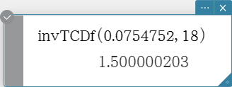
invTCDf

Returns the lower bound value of a Student’s t cumulative distribution probability for specified values.
Syntax: invTCDf (prob, df [ ) ]
Calculation Result Output: xInv

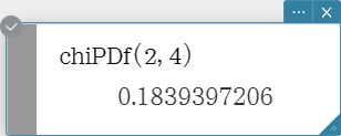
chiPDf

Returns the $ χ^2 $ probability density for specified values.
Syntax: chiPDf (x, df [ ) ]
Calculation Result Output: prob

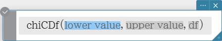
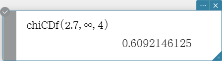
chiCDf

Returns the cumulative probability of a $ χ^2 $ distribution between a lower bound and an upper bound.
Syntax: chiCDf (lower value, upper value, df [ ) ]
Calculation Result Output: prob

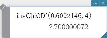
invChiCDf

Returns the lower bound value of a $ χ^2 $ cumulative distribution probability for specified values.
Syntax: invChiCDf (prob, df [ ) ]
Calculation Result Output: xInv

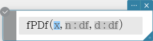
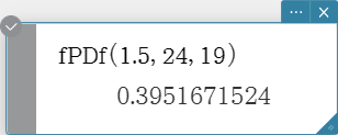
fPDf

Returns the F probability density for a specified value.
Syntax: fPDf (x, n:df, d:df [ ) ]
Calculation Result Output: prob

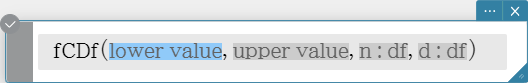
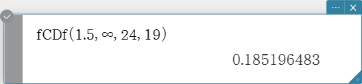
fCDf

Returns the cumulative probability of an F distribution between a lower bound and an upper bound.
Syntax: fCDf (lower value, upper value, n:df, d:df [ ) ]
Calculation Result Output: prob

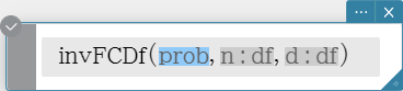
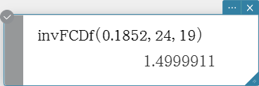
invFCDf

Returns the lower bound value of an F cumulative distribution probability for specified values.
Syntax: invFCDf (prob, n:df, d:df [ ) ]
Calculation Result Output: xInv

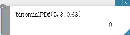
binomialPDf

Returns the probability in a binomial distribution that the success will occur on a specified trial.
Syntax: binomialPDf (x, numtrial value, pos [ ) ]
Calculation Result Output: prob

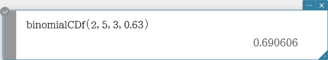
binomialCDf

Returns the cumulative probability in a binomial distribution that the success will occur between specified lower value and upper value.
Syntax: binomialCDf (lower value, upper value, numtrial value, pos [ ) ]
Calculation Result Output: prob

invBinomialCDf

Returns the minimum number of trials of a binomial cumulative probability distribution for specified values.
Syntax: invBinomialCDf (prob, numtrial value, pos [ ) ]
Calculation Result Output: xInv, *xInv

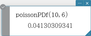
poissonPDf

Returns the probability in a Poisson distribution that the success will occur on a specified trial.
Syntax: poissonPDf (x, λ [ ) ]
Calculation Result Output: prob

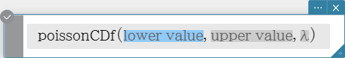
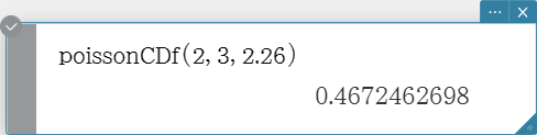
poissonCDf

Returns the cumulative probability in a Poisson distribution that the success will occur between specified lower value and upper value.
Syntax: poissonCDf (lower value, upper value, λ [ ) ]
Calculation Result Output: prob

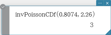
invPoissonCDf

Returns the minimum number of trials of a Poisson cumulative probability distribution for specified values.
Syntax: invPoissonCDf (prob, λ [ ) ]
Calculation Result Output: xInv, *xInv

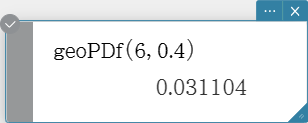
geoPDf

Returns the probability in a geometric distribution that the success will occur on a specified trial.
Syntax: geoPDf (x, pos [ ) ]
Calculation Result Output: prob

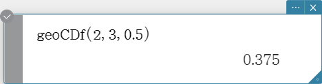
geoCDf

Returns the cumulative probability in a geometric distribution that the success will occur between specified lower value and upper value.
Syntax: geoCDf (lower value, upper value, pos [ ) ]
Calculation Result Output: prob

invGeoCDf

Returns the minimum number of trials of a geometric cumulative probability distribution for specified values.
Syntax: invGeoCDf (prob, pos [ ) ]
Calculation Result Output: xInv, *xInv

hypergeoPDf

Returns the probability in a hypergeometric distribution that the success will occur on a specified trial.
Syntax: hypergeoPDf (x, n, M, N [ ) ]
（$n$： Number of elements extracted from population、 $M$： Number of successes in population、 $N$： Number of population elements）
Calculation Result Output: prob

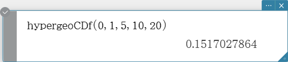
hypergeoCDf

Returns the cumulative probability in a hypergeometric distribution that the success will occur between specified lower value and upper value.
Syntax: hypergeoCDf (lower value, upper value, n, M, N [ ) ]
（$n$： Number of elements extracted from population、 $M$： Number of successes in population、 $N$： Number of population elements）
Calculation Result Output: prob

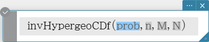
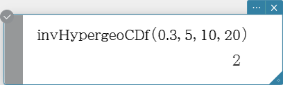
invHypergeoCDf

Returns the minimum number of trials of a hypergeometric cumulative distribution for specified values.
Syntax: invHypergeoCDf (prob, n, M, N [ ) ]
（$n$： Number of elements extracted from population、 $M$： Number of successes in population、 $N$： Number of population elements）
Calculation Result Output: xInv, *xInv

Источник

Normal Tools Overview

The Normal Tools give you several ways to set the Normals on objects in your scene. Methods include using a Helper object for aligning Normals, using a helper as a target for Normal vectors, tools for typing in specific Normal values, and functions to point normals out from common points like pivots and centers. There are also some helpful Normal selection tools to help speed up your work flow.

Normal Tools is now bundled with Wall Worm.

When you install the Normal Tools you’ll see a whole new rollout of functions when you add an Edit Normals modifier to an object. Those are added via a special custom attribute. The new rollout has functions that add extra functionality for selecting/setting normals. Working with foliage models for games is a lot easier with these functions.

Almost all functions include Macroscripts that can be utilized in custom scripts. The more that you understand Normals and the Edit Normals Modifier, the more you will appreciate the utilities in Normal Tools.

Inside the Normal Tools rollout (shown above right) you will notice a radio button labeled Apply To. This setting controls both the selection functions (at top) and the setting functions (below). Switch this setting when wanting to work on just the current selection or to the whole object. Most of the functions such as Out From/Element Out From have the same functions as explained in the Normal Tools Floater below.

Floater User Interface

Not only is there an extra rollout in new Edit Normals modifiers, there is also a floater for working on multiple objects at once and some extra functions that aren’t directly inside the Edit Normals custom attribute rollout. The Normal Tools UI is broken up into the following sections:

Helper Tape
Target
Normal Values
Set Normal Selection
Apply To
Auto Align from Object
Auto Align via Elements
Randomize

The use of these different sections are detailed in the following documentation.

Helper Tape

The Helper Tape is a standard Tape Helper that you can use for setting Normal directions.

Get Helper: Press this button to select the current Tape Helper in the scene. (If none exists for this session, a new Helper Tape will be created in the scene and selected. By default, this Tape will be positioned at the current selection center with a target pointing up in the Z axis (a normal vector of [0,0,1]).) This Tape will be used as the default Helper Tape until deleted or the Normal Tools floater is closed or re-opened.
Get Existing: Press this button to reuse an existing Tape Helper in the scene and set it as the current Helper Tape.
Move Helper to Picked Point: Press this button to bring up a Pick Point cursor. When you click a point in the scene, the Helper Tape will move to that location (but the target for the existing tape will remain at its current location). This function is useful for changing the normal direction without changing the current scene selection.

Target

This set of functions works with the Helper Tape’s Target.

Get: Press this button to select the Target for the normals. If no Helper Tape exists yet, a new one is created in the scene and its helper is selected.
Set Normal From: When pressed, the Normal Value (below) is updated to match the current direction of the Helper Tape based on the vector between the Helper Tape and the Target.
Move Target to Picked Point: When pressed, you can pick a point in the scene. Once picked, the Helper Tape Target will immediately move to that location. This function is useful for changing the normal direction without changing the current scene selection.

Normal Values

This set of functions allows you to set specific normal values as well as ways to derive normal values from other objects in the scene.

Up/Down Buttons

These two buttons set the current normal value to [0,0,1] (Up) or [0,0,-1] (Down). The Helper Tape Target will immediately match this normal vector.

Normal

This value is the current normal vector for edited normals when the Point Normals to Target is off. Valid formats for this value are:

[0,0,1]
[0 0 1]
0 0 1
0,0,1

To force the Helper Tape Target to match this vector, click the Set Helper Angle to Normal button (below).

Move Tape To Surface (default: On)

This option relates to the Get Normal From Surface function (below).

Get Normal From Surface

When pressed, you can pick a surface in the scene to derive the Normal from the picked surface. Once picked, the current Normal value (above) will be set to the surface normal picked. If Move Tape To Surface (above) is also on, then the Helper Tape is positioned at the picked point and the Target will match the surface normal.

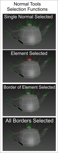
Set Normal Selection

This section gives you some tools for selecting Normals.

Wall Worm’s Normal Tools are a collection of utilities to make it easier to work with Normals inside 3ds Max. The tools are intended to fill the gap with some of the limitations with the current Edit Normals modifier included in 3ds Max.

Filter From Current Selection (default: Off): When On, the results of relevant selection functions will be limited to relevant normals that are a sub-set of the current set of selected Normals. For example, when on and the Select Border Normals is pressed, the resulting normals are only border Normals in the current selection. This option has no effect on the Invert Normals Selection function.
Select Border Normals: This button will set the current Normal Selection to only those Normals along the mesh’s border edges. This function can be bound to a keyboard shortcut with these macros in the wallworm.com category: Select Border Normals and Select Border Normals from Selection.
Select Element Normals (Version 1.4): This button will set the current Normal Selection to all Normals in the same geometric Element sub-object of the currently selected normals. This function can be bound to a keyboard shortcut with the Macro named Select Element Normals in the wallworm.com category.
Invert Normals Selections: This button will invert the current Normal Selection. Unlike using the CTRL+I shortcut, the node does not need to be in Normal sub-object mode.

Apply To:

The UI for the Apply To controls what objects/sub-objects are used for the Normal application functions; these tools also determine whether Normal changes are derived from the global Normal value in the Normal Values section or whether individual normals will point at the Helper Tape’s Target.

Apply To

This menu determines what normals on an object will update when the Apply Normal button is pressed. The options are explained below:

All Normals (default): All Normals in the object will update to point at the desired direction.
Selected Normals: Only normals currently selected in each object’s Normal sub-object mode will be updated. (When active, Live Target Mode is not available.)

Selection (default: On)

When on, the results of the Apply Normal function are restricted to the objects in the scene’s current selection. When off, only objects listed in the Objects to Edit list (below) are updated when Apply Normal is pressed.

Objects to Edit

By default, this list box is disabled. To enable, un-check the Selection check box.

When enabled, only those objects listed in this menu are used for the Apply Normal and Live Target Move results. Click the Add (+) button to add selected scene nodes to the list. Press the Remove (-) to remove the currently selected object from the list.

Point Normals to Target (default: Off)

When on, each edited normal will orient to point to the Helper Tape’s target. When off (default) the current Normal value is applied to all edited normals.

Apply Normal

When pressed, all relevant normals of all relevant objects (based on the current Apply To and Selection rules) will get updated to point at the new directions. The results are dependent on the Point Normals to Target option (above).

Live Target Move

This check button will turn on or off an active display of the normals on relevant objects. When on, changes to the current Normal or Helper Tape Target will immediately affect the normal results upon mouse-up (so moving the target will show targeted normals when the move is finished). At this time, this mode only supports an Apply To set to All Normals.

Stitch Colocated Normals

This function will average the vector of all normals derived from the same location. This is helpful for border normals that are not smoothed because their smoothing groups don’t work for unwelded vertices.

Offset Origin (Version 1.47)

This function is not available from the Normal Tools floater. This function is only present in the Normal Tools rollout of an Edit Normals modifier.

When the Use Offset Origin setting is on, the point from wich normals are derived from will be offset in orld space by the offset value. This is helpful when using functions like Out From Element Bottom, for example. In this case, if an Origin Offset value of [0,0,-16] is set, then the bottom point will be offset by -16 units in the world Z axis.

Out From Object

These functions allow you to quickly align the normals across an object in a way that is often helpful for foliage.

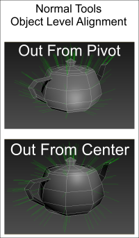
Pivot (Version 1.2): When pressed, aligns all pivots out from the node pivot to the vertex.
Center (Version 1.2): When pressed, aligns all pivots out from the node’s center to the vertex.
Face (Version 1.1): When pressed, the normals will align to the vector defined by the face center to the point from whence the normal originates. The results are dependent on the type of object being applied to: For Editable Poly objects, the normal aligns from the Polygon’s Safe Center. For all other objects, the normal aligns from the Tri (face) center. Generally speaking, using Editable Poly is prefered.

Elements Out From

All of these buttons align the normals per Element sub-object.

Centers(Version 1.4): When pressed, aligns all pivots out from the element center.
Bottom (Version 1.4): When pressed, aligns normals from the bottom-most center of the element to the vertices in the Object’s coordinate system.
Base (Version 1.4): Similar to Bottom, this will align the normals with a vector from the bottom-most vertex in the element out to all the other vertices
Near Pivot (Version 1.4): When pressed, aligns normals in each element from the vertex in that element that is closest to the pivot of the object.
Near Center (Version 1.4): When pressed, aligns normals in each element from the vertex in that element that is closest to the center of the object.

Some of the Element-level alignment functions may not work well with some geometry, especially when there are several vertices that are equally valid for choosing a bottom or closest-to object center or pivot. Generally, the Align from Center and Bottom are the most appropriate for general useage. The others often require using the Apply To: Selected Only option.

From Helper (Version 1.47)

If a helper object is assigned, the normals will all radiate from the pivot point of the helper object.

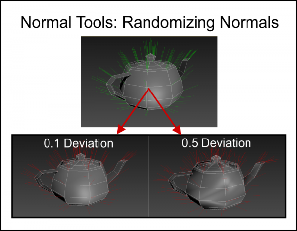
Randomize

The Randomize function will randomly deviate the affected normals from their current vector based on the allowed randomize range. A low value will deviate the normals slightly. A high value (like 0.5) will create significant deviation. A value of 1.0 will make all normals completely random (and is probably not what you expect).

Requirements

You must own 3ds Max to use this tool set. To date, it has been tested in 3ds Max 2012-2021.

Installation & Upgrading

If you use the general Wall Worm Model Tools, Wall Worm Pro or Wall Worm Pro Pack, you should just install the latest version of that tool because Normal Tools is now included with that installation. Otherwise, you can install manually with the steps below:

To install, copy the file named wallworm_normals.mse from the download file into your Scripts\Startup folder inside 3ds Max and restart 3ds Max.
Copy the file named LaunchNormals.mcr from the downloaded zip onto your computer.
In Max, click MAXScript > Run Script… and browse for the LaunchNormals.mcr that you copied.
You must then add a menu or button to launch the tools via Customize > Customize User Interface and choose Wall Worm Normal Tools under the wallworm.com category.

Known Issues

Using instanced Edit Normals modifiers is not fully supported with the Apply Normal function.
In some versions of 3ds Max, you cannot select in the viewport a Tape Helper that was created by MAXScript. If this affects you, use the Get Helper button in the Normal Tools UI or use the Layer Manager.

Explicit Normals and Wall Worm

Many people who use Wall Worm for the Source Engine are suprised to find out that you can edit normals in any other method than using Smoothing Groups. Using the Edit Normals modifier will translate into your game’s model as long as you are using the WW SMD Exporter and your WWMT settings have the Explicit Normals (and sometimes Auto) set for the Normals at export-time. See Export Correct Smoothing on Models.

Resources

Understanding the Edit Normals Modifier is key in using this tool. Here are some useful topics that may help you understand using Edit Normals more effectively.

Edit Normals Modifier
Smoothing and Hard Edges from Polycount
Eric Chadwick on Tree Shading

Источник

One fundamental interpretation of the derivative of a function is that
it is the slope of the tangent line to the graph of the
function. (Still, it is important to realize that this is not
the definition of the thing, and that there are other possible and
important interpretations as well).

The precise statement of this fundamental idea is as follows. Let $f$
be a function. For each fixed value $x_o$ of the input to $f$, the
value $f'(x_o)$ of the derivative $f’$ of $f$ evaluated at $x_o$ is
the slope of the tangent line to the graph of $f$ at the
particular point $(x_o,f(x_o))$ on the graph.

Recall the point-slope form of a line with slope $m$ through a
point $(x_o,y_o)$:
$$y-y_o=m(x-x_o)$$
In the present context, the slope is $f'(x_o)$ and the point is
$(x_o,f(x_o))$, so the equation of the tangent line to the graph
of $f$ at $(x_o,f(x_o))$ is
$$y-f(x_o)=f'(x_o)(x-x_o)$$

The normal line to a curve at a particular point is the line
through that point and perpendicular to the tangent. A person
might remember from analytic geometry that the slope of any line perpendicular to a line with slope $m$ is the negative
reciprocal $-1/m$. Thus, just changing this aspect of the equation
for the tangent line, we can say generally that the equation of
the normal line to the graph
of $f$ at $(x_o,f(x_o))$ is
$$y-f(x_o)={-1\over f'(x_o)}(x-x_o).$$

The main conceptual hazard is to mistakenly name the fixed point
‘$x$’, as well as naming the variable coordinate on the tangent
line ‘$x$’. This causes a person to write down some equation which,
whatever it may be, is not the equation of a line at all.

Another popular boo-boo is to forget the subtraction $-f(x_o)$ on the
left hand side. Don’t do it.

So, as the simplest example: let’s write the equation for the tangent
line to the curve $y=x^2$ at the point where $x=3$. The derivative of
the function is $y’=2x$, which has value $2\cdot 3=6$ when $x=3$. And
the value of the function is $3\cdot 3=9$ when $x=3$. Thus, the
tangent line at that point is $$y-9=6(x-3)$$ The normal
line at the point where $x=3$ is
$$y-9={-1\over 6}(x-3)$$

So the question of finding the tangent and normal lines at various
points of the graph of a function is just a combination of the two
processes: computing the derivative at the point in question, and
invoking the point-slope form of the equation for a straight line.

Exercises

Write the equation for both the tangent line and
normal line to the curve $y=3x^2-x+1$ at the point where $x=1$.
Write the equation for both the tangent line and
normal line to the curve $y=(x-1)/(x+1)$ at the point where $x=0$.

Источник

Abbreviations and Punctuation Used in This Section

Trigonometric and Inverse Trigonometric Functions

Hyperbolic and Inverse Hyperbolic Functions

Angle Units

Mixed Fraction

Logarithmic Function

Numeric Calculations

signum

Int

frac

intg

fRound

sRound

Random Number Generator

rand

randList

randNorm

randBin

RandSeed

Integer Functions

iGcd

iLcm

iMod

Permutation and Combination

nPr

nCr

Other Functions

judge

piecewise

isPrime

with Operator ( | )

delta

\(n\)th-delta

heaviside

gamma

strToExp

Transformation

approx

simplify

expand

factor

rFactor

factorOut

combine

collect

tExpand

tCollect

expToTrig

trigToExp

toFrac

propFrac

dms

toDMS

Advanced

solve

dSolve

taylor

laplace, invLaplace

fourier, invFourier

FFT, IFFT

Calculation

diff

impDiff

Integrate

lim

sum

prod

rangeAppoint

mod

tanLine

normal

arcLen

fMin, fMax

gcd

lcm

denominator

numerator

Complex

arg

conjg